Top-Down Analysis in Technical Analysis

Top-down analysis begins with a study of the major markets such as interest rates, currencies, commodities, and stock market to determine which market has the highest possibility of profit in the future. Once a market has been selected, the next level of decision making is the groupings of issues in that market and, finally, the individual issues within those groupings. In the currency markets, the breakdown for U.S. investors is basically whether to invest in the dollar or in a foreign currency. If it is to be a foreign currency, the selection is large and can be broken into further groups—for example, the resource-producing countries and the emerging countries. If the bond market is chosen, the groupings can be on length to maturity, country and currency, and level of default risk. In the stock market, of course, industry groups are the standard sectors, but others are used such as capitalization, foreign origin, investment style, and interest-rate related. First, though, the investor must decide the long-term, secular trend in the various markets. As in trading, the trend is the most important aspect of any price change and the major determinant of whether the investor will profit from investing. Bucking the trend in investing is just as dangerous as it is in trading.

The technical method used to determine markets’ relative attractiveness is called ratio analysis. It compares different markets with each other to see which is performing most favorably. After a market has been selected that fits the investor’s objectives, further comparisons are made with components of that market, such as by industry group, capitalization, or quality.

1. Secular Emphasis

John Murphy, in his book Intermarket Technical Analysis (1991), discussed the concept of alternating emphasis in the markets on hard assets and soft assets over long secular periods. Secular is a term used for any period longer than the business cycle. Hard assets are solid commodities such as gold and silver; these assets traditionally are considered an inflation hedge. Soft assets are financial assets, called paper assets, which primarily include stocks and bonds.

The reason for the inverse relationship between the value of hard assets and of soft assets is that a close correlation exists between material prices and interest rates. Inflation, or higher material prices, is generally associated with higher interest rates. When inflation becomes a threat, paper assets, which decrease in value as interest rates rise, are undesirable as investments. Likewise, when hard asset prices decline, interest rates usually decline, and soft assets increase in value. The theory that one or the other of these kinds of assets becomes popular for substantial periods is not a new one.

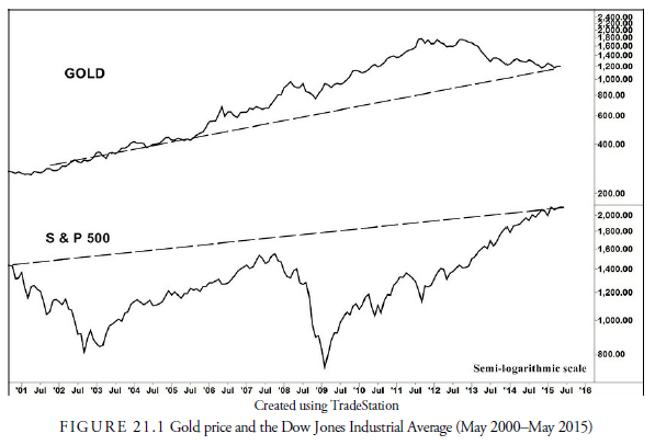
As the theory states, when hard assets rise in value, soft assets decline. However, between 1998 and 2012, this relationship has not always held. Gold is traditionally the measure of hard asset prices because of its universal appeal as an inflation hedge, and the stock market is a soft asset. Figure 21.1 shows the history of gold prices and the Dow Jones Industrial Average since 2000. Except during the major decline in stock prices from 2000 through 2009 and a few other “bumps,” these two markets uncharacteristically headed in the same directions. Indeed, over this period, gold outperformed the stock market. This action dispels the theory that they will travel in opposite directions.

Looking at a ratio chart of gold to the stock market, we see that clear trends develop in the relationship between these two types of assets. Figure 21.2 shows a graph of the ratio of gold to the stock market. A decline in the gold/stock market ratio indicates that gold is underperforming the stock market and, in relationship to the stock market, is not a wise investment.

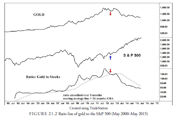
In this case, the broad signal as to when to switch from one asset class to another is given when the ratio crosses its 24-month SMA. This is a crude method of signaling and requires considerable refinement but here is used for illustrative purposes. In Figure 21.2, the last signal to switch from hard assets to soft assets occurred around May 2012 when gold was trading at 1,300/oz. and the S&P 500 was around 1,585. Until then, gold had been outperforming stocks.

Although these signals are not precise by any means, they do indicate over long periods in what asset type the investor should be invested. Once a definite trend toward one or the other asset type is clear, it usually remains in place for many years.

Even though we have used gold as an example of a hard asset thus far, gold is not necessarily the best hard asset. Others exist, such as silver, oil, copper, and aluminum. These are called industrial raw materials or industrial metals and are normally associated with the business cycle. An increase in industrial metals prices generally indicates business expansion. Along with gold, these industrial prices have a long-term component that coincides with the gold price and gives more options for investment during a period of hard assets.

Figure 21.3 shows the relationship between industrial metals prices and the stock market since 2005. We used old-fashioned trend lines for signals, and the last one in March 2012 coincided almost exactly at the sell signal for gold.

What does this mean for investment selection? Being in the time period following the 2012 signal for the switch to soft assets suggests that analysis should be concentrated on those investments concerned with the stock market or bond market.

2. Cyclical Emphasis

Within the longer secular economic trend are a number of business cycles. These business cycles are of varying length but usually average around four to five years. These business cycles are the normal horizon for most economists, business managers, and investors. It is well recognized that leadership in the trading markets often switches within the business cycle. There appears to be a standard pattern that is worth watching. Murphy maintains that although the markets may appear independent, they are interrelated and follow certain patterns. For that reason, he suggests that investors should be aware of all these markets and their interactions. The activity in all of these markets might offer suggestions about investment prospects.

Martin Pring (2002) classifies investment markets into three categories: commodities, bonds, and stocks. Murphy adds currencies and, to some extent, foreign stock markets, to this list. The business cycle affects each of these markets but in different ways. Let us look at the normal sequence of leadership among these investments and see how to recognize when a change in leadership has occurred. We will look in sequence at the dollar exchange rate to gold, using gold as a proxy for inflation and commodity prices, gold futures contract to the long-term bond (U.S. Treasury 30-year futures contract), a proxy for interest rates, the long­term bond to the stock market (Standard & Poor’s 500), and, finally, the stock market back to the dollar exchange rate (U.S. Dollar Index—DXY).

Murphy maintains that currency rates influence industrial prices but sometimes with a considerable lead. The dollar is important in that it is the pricing currency for many of the world’s raw materials such as oil, gold, and other precious metals. When the dollar declines, it makes these commodities cheap in foreign currencies but expensive in dollar terms. Thus, there is a leading inverse relationship between the U.S. dollar and raw materials prices in the United States. In Figure 21.4, we use gold as a proxy for industrial prices because gold has a well-defined price, whereas most indexes of material prices have different weightings for their components and are, thus, biased toward the interest of the respective index compilers. Figure 21.4 shows the ratio of the dollar to gold and gold itself. When the ratio is rising, or the dollar is stronger than gold, gold tends to decline, and vice versa.

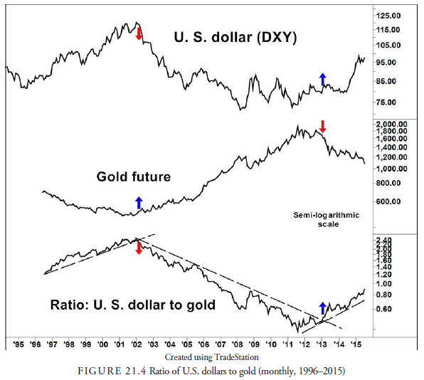
We use the trend line as the means of generating a crossover signal. In Figure 21.4, the most recent ratio line crossed upward through a trend line in December 2011, suggesting a rise in the dollar versus gold. At that time, the dollar was in a long downward trend, blocking any purchase until it turned up in August 2014 when it broke upward through its own downward trend. This raises an important point about investing on ratios. Because a ratio can be tilted one way or the other even when both components are declining, the investor must never enter the favored market until it also is advancing on an absolute basis. In the current instance, although the dollar was favorably compared to gold, it should not have been bought until August 2014 when it finally turned up. Had it not turned up and then underperformed gold later, the investor would have saved his portfolio from loss in each asset class by not acting based solely on the ratio crossover.

3. Gold and Bonds (Long-Term Interest Rates)

The next sequence is typically for industrial prices to lead long-term U.S. interest rates. This was not the case in the period between 2005 and 2012 when both asset classes rose, gold outperforming bonds. Thus, the assumed relationship did not occur, raising questions about future assumed relationships. It doesn’t help portfolio performance by arguing that the FED kept interest rates low and thus upset the normal relationship. Excuses don’t save money, but research, flexibility, and skepticism do.

By taking a ratio of the gold price to the U.S. Treasury bond futures, we see that at certain times, a signal is given by the ratio as to when to enter or exit the long-term bond market. The ratio is shown in Figure 21.5. The most recent signal of trend change is occurring at the time of this writing, June 2015, and like many signals, it is not yet clear. The reason is that the upward crossover in the ratio is not confirmed yet by an upward crossover in the favored gold price. On the other hand, the bond market is edging slightly below its upward trend line and is in a position to be sold. The bottom line is that the gold futures need to progress higher to confirm their relative strength, but bond futures can likely be sold right now.

4. Bond Market and Stock Market

Ideally, in the normal business cycle sequence, the next switch in markets is from the bond market to the stock market. As Chapter 10, “Flow of Funds,” demonstrated, the lead-lag relationship has not been a successful one since 1998. Murphy argues that this is because for the first time since the 1930s, actual deflation has become a threat and has upset the previous balance between interest rates and the stock market. Nevertheless, a plot of the ratio of bonds to stocks, as shown in Figure 21.6, shows definite times when one or the other has the advantage.

The ratio in Figure 21.6 shows wide swings in the relationship between stocks and bonds. From after the 2003 stock market bust, stocks outperformed bonds handily. However, in November 2007, almost at the peak of the stock market, the ratio turned up, suggesting that stocks be sold in favor of bonds. And again, at the bottom of the market crash, the ratio swung the other way and suggested a return to the stock market again. This suggests that the bond to stock ratio has an excellent history of timing the stock market.

5. U. S. Dollar and the Stock Market

The final analysis is to return to the beginning and see how the dollar and the stock market have interacted. The dollar usually leads the industrial raw material market, which in turn generally leads the bond market, which in turn leads the stock market. By connecting the loop, nothing is accomplished because there seems to be only a slight relationship between the stock market and the dollar. This may have changed also, because Figure 21.7 shows the dollar now has an excellent timing relationship with the stock market. The dollar to stocks ratio gave a buy signal for the dollar and a sell signal for the stock market in December 2007, right at the peak in the stock market. Roughly a year later in March 2009, the reverse occurred when the ratio suggested a switch from the dollar back into stocks, right at the stock market bottom.

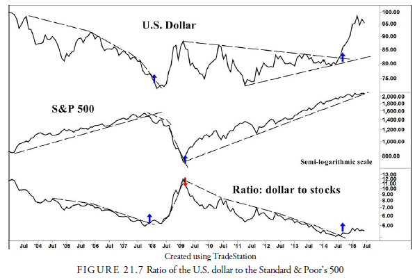
A little disconcerting right now is that the signal occurred again to buy the dollar and sell the stock market in September 2014. As of this writing, the stock market has not confirmed the signal by breaking its trend, but the dollar is completing a strong rally.

6. Implications of Intermarket Analysis

From the previous analysis, it appears that around 2001, the investor should have been looking at the raw materials markets and the stock market. Because both markets appeared favorable, the raw material market stocks would likely have been the best investments. The signals given by the various ratios are usually long­term signals, in the sense that they are operating within the business cycle. They are neither trading signals nor mechanical signals. Their purpose is to inform the investor in which markets to invest solely from the way the marketplaces are behaving. When certain sectors become strong, they tend to remain strong, just as when a trend begins, it tends to remain. Eventually these ratios will suggest changes in the investment mix, but only rarely do they err, and often that miscalculation comes from the investor impatience and greed, treating the signals as mechanical rather than waiting to be sure they are real.

7. Create an Array

One method of consolidating all the relationships mentioned earlier and lessening the difficulty in keeping straight the current situation with these asset classes is to periodically draw an array that includes the classes and gives a hint as to where investment assets should most likely be placed. In Table 21.1 is an array of the current readings of the preceding charts and their summary.

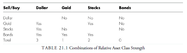
The array in Table 21.1 suggests that investments should be half invested in dollar assets and none in the bond market, leaving a split between gold and the stock market, with more emphasis on the stock market. Investments in dollars suggests selling foreign currencies and buying dollar-producing entities such as companies that produce overseas and sell exclusively to Americans. The point in this exercise of determining what asset classes have the most promise during the business cycle is to provide a framework for determining with some degree of certainty just where investment funds should go. Once the overall plan is established, the nitty-gritty of deciding of sectors, groups, and so on becomes a study of specific areas for direct investment. At that point, the analyst can use his technical skills to sort out the issues worth playing.

Finally, this analysis is not intended to forecast the economy. It is useful primarily in determining where the best market for investment might be at any time. Because most indicators lead the economy, forecasting the economy is unfruitful. From this information, certain aspects of the economy are obvious, but investment is best left to the analysis of price than to the analysis of the lagging economy.

Box 21.1 Law of Percentages

A relative loss of 20% can be made back with a relative gain of 20%, but an absolute 20% loss requires a 25% gain to break even. This is called the law of percentages. In investing, it suggests that all absolute losses must be kept to a minimum. As the old adage goes, “You can’t spend a relative return.” For example, if you have $100 in capital and sustain a 20% loss, you are left with $80. You must earn a 25% return on the $80 to return to the break-even level of $100. For any particular loss amount, the percentage amount that must be gained to break even is calculated using the formula %gain necessary = %loss ^ (1 – %loss). As an extreme example, a 50% loss requires a 100% gain to break even. Considering the difficulty of investing for a 100% gain, the investor is better off cutting losses before reaching such an extreme that is unlikely to be recouped.

8. Stock M arket In dustry Sectors

Should the stock market become a potential favorite from the business cycle analysis above, the next step is to either go downstream to industries or groups and then to specific issues or just start at the bottom with stocks and let their strength tell the investor where the opportunities lie. On the former method, some analysts have proposed theories of industry group and sector rotation during the stock market cycle. These rule definitions, however, are too strict, and often the markets do not accommodate them. For example, some models suggest that utilities, generally considered interest-related stocks, should be bought at certain stages of the market cycle when interest rates are expected to decline. However, as we have seen previously, when an inflationary environment exists, anything to do with interest rates will generally underperform. In other words, any system of following specific models of business cycles is not flexible enough to account for changes in the major market segments.

For some individuals, like stock mutual fund managers, investment in the stock market is a requirement. In these instances, the best manner of screening out the most likely sectors to outperform is the use of ratio analysis between the sector performance and the stock market as a whole. For example, Figure 21.8 shows a three-point reversal, point and figure plot of the Dow Jones Utilities Sector to the Dow Jones Industrials. Figure 21.9 shows a three-point reversal, point and figure plot of the Dow Jones Energy Sector to the Dow Jones Industrials.

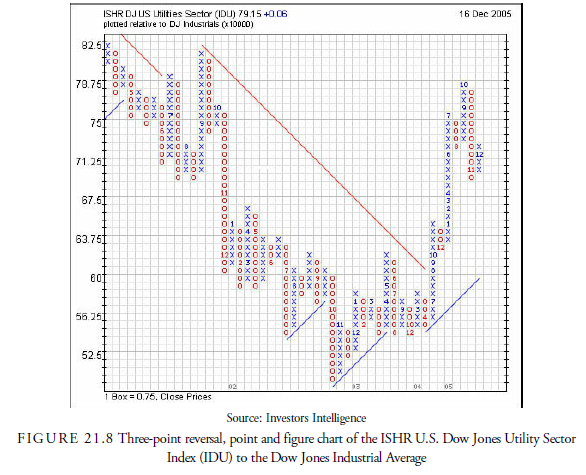
Plotting the relative strength ratio of an industry and often a stock to some underlying average, we often see an irregular line that is difficult to interpret. By plotting these ratios on a point and figure chart, the minor, less significant oscillations are eliminated, and the overall relationship of the two indices becomes more obvious. In Figure 21.8, for example, it is clear that underperformance of utility stocks began in 2009. These charts are much more informative than a line chart. Remember, however, when deciding whether to act on any of the ratio analyses, the absolute price action of the stock in the numerator always must be analyzed as well. When both charts demonstrate a trend, one can act with more confidence.

Source: Kirkpatrick II Charles D., Dahlquist Julie R. (2015), Technical Analysis: The Complete Resource for Financial Market Technicians, FT Press; 3rd edition.