Two Group Analysis in Full Structural Models

A two group analysis can see if differences exist in the relationships proposed in a model across groups. Performing a two group analysis is very similar to the discussion about measurement invariance in Chapter 4. Let’s continue with the example used in the full structural analysis of Adaptive Behavior and Servicescape leading to Customer Delight, which influences Positive Word of Mouth and Tolerance to Future Failures. The example going forward is for a full structural analysis, but the exact same process can be used for a path model. After initially drawing out your model in AMOS, you need to specify the two groups. For this example, the two groups will be (1) new customers and (2) repeat customers. We will see if first-time customers differ in their evaluation and atti- tudes compared to repeat customers who have been through the experience before. In the “Models” window, the default value will be one group labeled “Group 1”. We need to create two groups for the analysis. The first step is to rename the “Group 1” label to something meaningful. To do this, you need to initially double click in this Group 1 label. A pop-up “Manage Groups” window will appear where you can change the name of the group. Let’s call the first group “First_Time” to represent the first-time customers. You will then need to hit the “New” button at the bottom of the manage groups pop-up win- dow to form another group. Let’s call the second group “Repeat” to represent the repeat customers.

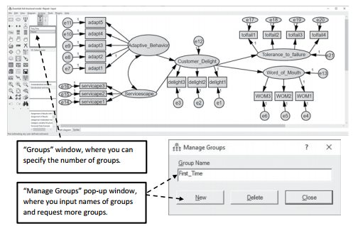
Figure 5.23 Setting Up Two Groups in a Structural Model

After forming the groups, you need to specify where the data is for each group. Each group can have a separate data file or can be in the same data file, but you will need to specify the values of each group for AMOS. Hit the  “Data Files Button” and then select the “File Name” button and find your data file. For this example, the file name is called Customer Delight Data. In this file, I have a col- umn called “experience” that is populated with a 1 or a 2 value.The “1s” denote repeat customers and the “2s” denote first-time customers. If you are using the same data file for both groups, you will need to use the “GroupVariable” function to tell AMOS what column the group differences are in.You will also have to tell AMOS what value corresponds with which group using the “GroupValue” button.

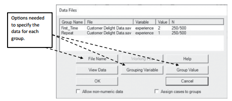
Figure 5.24 Reading in the Data File for Each Group in the Analysis

In this example, we have an even split of the total 500 sample.With a two group analysis, you need to make sure each group has a sufficient sample size to accurately capture the relationships within each group. This can be a downside with two group analyses because each group has to have a sufficient sample for power reasons, which means the overall sample size can be quite large. After reading in the data file for each group, you need to hit the “OK” button.To run a two group analysis, you will have to label every parameter and error term for each group.AMOS has a function for this so that you do not have to label everything individually.You will need to use the “Multi-Group” analysis button, which looks like a double headed icon .After selecting this icon, you will initially get a pop-up warning window.This warning window is just stating that it is going to set up potential models to test in AMOS and, if existing models are already set up, AMOS will delete those previous models. In essence, it is going to start with the default models of a two group comparison.

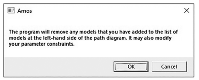
Figure 5.25 Warning Message Using Multiple Group Analysis

Select the “OK” button on this warning window. Next, a pop-up “Multiple-Group Analysis” window will appear and will let you know what potential models are being suggested to test. The type of model AMOS will suggest will depend on the complexity of your model. In this example, AMOS suggested five potential models. The checkmarks in this pop-up window denote if you want these different parameters constrained to be equal across the groups. I usu- ally just hit “OK” and let AMOS create the models even if I am not going to use that specific model. It takes more time to deselect the parameters you do not need. If I have extra models I do not need, I just ignore that output.

After hitting “OK”, you will see in the models window an unconstrained model across the two groups, and then you will see five different models that are constraining the two groups.

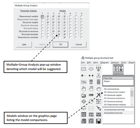
Figure 5.26  Comparison Models in Multiple Group Analysis

Figure 5.27 Unique Parameter Labeling for Each Group

In a two group analysis, if you use the multigroup analysis icon to label your parameters across the groups, AMOS will use an “a” and a number for factor loadings and a “b” and a number for structural relationships between constructs. It is very important that every parameter has a unique name across the groups. For instance, the structural relationship from Servicescape to Customer Delight is labeled “b3_1” for the first-time customer group and “b3_2” for the repeat customer group. This similar notation lets you know that “b3” is the specific relationship from Servicescape to Customer Delight but the underscore numbers after “b3” lets you know which group for clarification purposes.

In Chapter 4, we talked about how to test for invariance, and specifically metric invariance was a test of factor loadings being constrained across the groups. The measurement weights model in AMOS specifically constrains all factor loadings (or parameters listed as an “a”) to be equal across the groups. The structural weights model constrains the factor loadings but also constrains the relationships between constructs to be equal. If you double click into the structural weights model on the graphics screen, you will see the measurement and structural relationships constrained. See Figure 5.28.

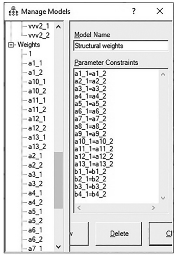
Figure 5.28 Parameters Constrained to be Equal Across the Groups

If we run the two group analysis with the structural weights model, this will tell us if first- time and repeat customers are different as a whole.This analysis is examining all of the relation- ships in the model across the groups. If we find differences in this model, it tells us only that the groups are significantly different as a whole; it gives us no indication exactly where in the model they are different.You might have one relationship that is extremely different across the groups and all other relationships were non-significant. When you examine the relationships as a whole, you cannot tell where in the model any differences are coming from. Hence, we need to form a new model that is not a default model listed by AMOS. In the models window, if you double click on the last model “Measurement Residuals”, the managed models pop-up window will appear. At the bottom of the window is a button called “New”. Select this button, and a new model will be created that is currently blank.You need to first title this model. We are going to call this model “Constrain 1”. Next, we constrain one structural relationship at a time to see if the specific relationship is different across the groups. Remember that structural relationships are labeled as “b” and a number in AMOS. Let’s look at the first structural rela- tionship of Adaptive Behavior to Customer Delight.

Figure 5.29 Adaptive Behavior to Customer Delight Constrained to be Equal Across the Groups

This relationship is labeled as b1 (b1_1 for first-time customers and b1_2 for repeat customers). We need to constrain this specific relationship to be equal across the groups to see if differences are present. In the “constrain 1” model, you are going to constrain b1_1 to be equal to b1_2. Note if you double click on the value listed in the left-hand menu, it will automatically include this in the parameter constraint window. After constraining this relationship to be equal across the groups, hit the close button, and then we are ready to run the analysis. Once the analysis has finished, you first go to the Model Comparison link in the output. This will tell you if there is a difference in chi-square values across your models. The output in this section will show comparisons of the different models listed. In the first section, you will see a subheading that says, “Assuming model Unconstrained to be correct”. This compares all the constrained models listed by AMOS to the unconstrained model where no relationships were constrained to be equal. In this first section, we are concerned with the “Constrain 1” model, where we are testing the relationship from Adaptive Behavior to Customer Delight.

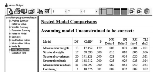
Figure 5.30 Model Comparison Results

The results of the “Constrain 1” model show that the chi-square difference for the one parameter that we constrained is 10.57, which is a p-value at the .001 level (Remember that with one degree of freedom, significance at the .05 level requires a chi-square value of at least 3.84).These results for the Constrain 1 model mean that the relationship of Adaptive Behavior to Customer Delight is significantly different across the groups. Now that we know a signifi- cant difference is present, we need to see which group has a stronger or weaker effect on the relationship. To do this, we need to go to the Estimates link in the output. In the Estimates output, we are going to examine the strength of the relationships across the two groups.There is a “Groups” window on the left-hand side of the Estimates output.You need to first select the group you are interested in, and this will present the relationships for that specific group. See Figures 5.31 and 5.32.

Figure 5.31 Estimates Output for First-Time Group

Figure 5.32 Estimates Output for Repeat Group

If you look at the Adaptive Behavior to Customer Delight relationship across both groups, you will see that the first-time customers have a much stronger relationship than the repeat customers. Thus, we can conclude that adapting a service for a first-time customer has a sig- nificantly stronger influence on Customer Delight than with repeat customers.You can see the standardized regression weight for first-time customers (.650) is substantially stronger than with repeat customers (.376).

If you would like to test the next relationship of Service- scape to Customer Delight (labeled as b3), then go back into the “Constrain 1” model on the graphics page and replace the b1 constraint for a b3 constraint. After you do this, close the window and run the analysis again.The first step is to go to the output sec- tion and examine the model comparison output again. This will let you know if you even have a significant difference across the groups for this spe- cific relationship.

Figure 5.33 Servicescape to Delight Constrained

Figure 5.34 Model Comparison Results for Constrained Relationships

The results of this test (Constrain 1) show that there is no significant difference between the groups for the Servicescape to Customer Delight relationship (∆c2/1df = 0.663). Thus, the groups are very similar in its relationship from Servicescape to Customer Delight.To fully understand the differences across the groups, you will need to individually constrain all the other relationships in the model.With a big model, this can be tedious to individually test each relationship, but it is necessary to see exactly where differences lie across the groups.

Another option instead of testing one relationship at a time is to create a separate model test for each structural relationship in the model. By doing this, you can see the differences across groups for every structural relationship at once instead of running the same test over and over. For instance, in our example, we have four structural relationships.We could create four additional model tests, and instead of calling the structural test “Constrain 1”, we can call the test “b1 test”, “b2 test”, “b3 test”, and “b4 test”. With the b1 test, we would constrain b1_1 = b1_2.We would repeat this with each of the structural tests.

Figure 5.35 Constraining Every Structural Path Across the Groups

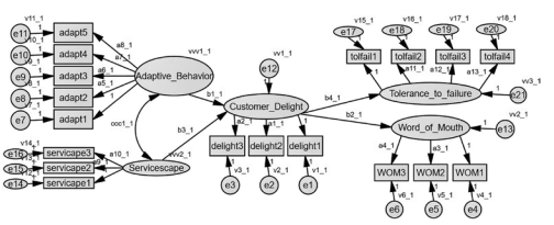
Figure 5.36 Example of a Full Structural Model Labeled

After creating a separate model test for each structural relationship, you are now ready to run your analysis and go back to the model comparison output. In the output, you can see the individual structural relationships that are tested (b1–b4).

Figure 5.37  Model Comparison Results With Individual Structural Paths Constrained

Now we can see all the structural relationship tests at once. We see that b1 and b4 are sig- nificantly different across the groups, but b2 and b3 are non-significant. As stated before, you would need to go back into the Estimates output to see which relationship is stronger or weaker across the groups.

Figure 5.38 Model Fit Results for Multiple Group Analysis

One last thing we need to address is model fit statistics with our two group analysis. If we go into the Model Fit output, we do not get fit statistics for each group. With a two group analysis, AMOS will give you a model fit across the two groups. It examines how the model fits the data in the presence of both groups. In the output, we are only concerned with the “Unconstrained” model fit statistics. This is assessing model fit across both groups. All other model fit statistics are not that helpful in a two group analysis.

Source: Thakkar, J.J. (2020). “Procedural Steps in Structural Equation Modelling”. In: Structural Equation Modelling. Studies in Systems, Decision and Control, vol 285. Springer, Singapore.