Using Logistic Regression with Stata

Here is the same regression seen earlier, but using logistic instead of logit:

. logistic any date

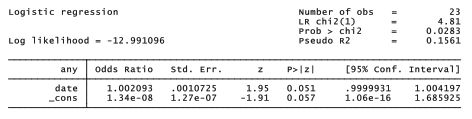
Note the identical log likelihoods and %² statistics. Instead of coefficients (b), logistic displays odds ratios (e^b ). The numbers in the Odds Ratio column of the logistic output are amounts by which the odds favoring y = 1 are multiplied, with each 1-unit increase in that x variable (if other x variables’ values stay the same).

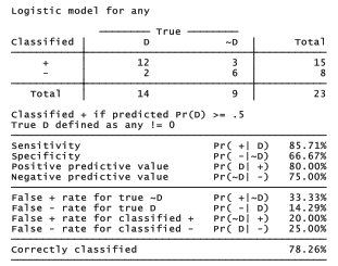
After fitting a model, we can obtain a classification table and related statistics by typing . estat class

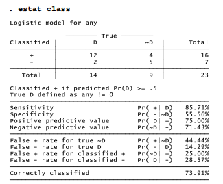
By default, estat class employs a probability of .5 as its cutoff (although we can change this by adding a cutoff( ) option). Symbols in the classification table have the following meanings:

D        The event of interest did occur (that is, y = 1) for that observation. In this example, D indicates that thermal distress occurred.

~D        The event of interest did not occur (that is, y = 0) for that observation. In this example, ~D corresponds to flights having no thermal distress.

+           The model’s predicted probability is greater than or equal to the cutoff point. Since we used the default cutoff, + here indicates that the model predicts a .5 or higher probability of thermal distress.

– The predicted probability is less than the cutoff. Here, – means a predicted probability of thermal distress below .5.

Thus for 12 flights, classifications are accurate in the sense that the model estimated at least a .5 probability of thermal distress, and distress did in fact occur. For 5 other flights, the model predicted less than a .5 probability, and distress did not occur. The overall correctly-classified rate is therefore 12 + 5 = 17 out of 23, or 73.91%. The table also gives conditional probabilities such as sensitivity or the percentage of observations with P > .5 given that thermal distress occurred (12 out of 14 or 85.71%).

After logistic or logit, the postestimation command predict calculates various prediction and diagnostic statistics. Explanations for logit model diagnostic statistics can be found in Hosmer and Lemeshow (2000).

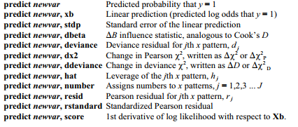
Statistics obtained by the dbeta, dx2, ddeviance and hat options do not measure the influence of individual observations, as do their counterparts in ordinary regression. Rather, these statistics measure the influence of covariate patterns; that is, the consequences of dropping all observations with that particular combination of x values. See Hosmer and Lemeshow (2000).

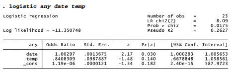
Does booster joint temperature also affect the probability of any distress incidents? We could investigate by including temp as a second predictor variable.

Including temperature as a predictor slightly improves the correct classification rate, to 78.26%.

. estat class

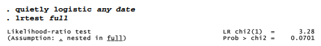
According to the fitted model, each 1-degree increase in joint temperature multiplies the odds of booster joint damage by .84. In other words, each 1-degree warming reduces the odds of damage by about 16%. Although this effect seems strong enough to cause concern, the asymptotic z test says that it is not statistically significant (z = -1.476, p = .140). A more definitive test, however, employs the likelihood-ratio /². The lrtest command compares nested models estimated by maximum likelihood. First, estimate a full model containing all variables of interest, as done above with the logistic any date temp command. Next, type an estimates store command, giving a name (such as full) to identify this first model:

. estimates store full

Now estimate a reduced model, including only a subset of the x variables from the full model. (Such reduced models are said to be “nested.”) Finally, a command such as lrtest full requests a test of the nested model against the previously stored full model. For example (using the quietly prefix, because we already saw this output once),

This lrtest command tests the recent (presumably nested) model against the model previously saved by estimates store. It employs a general test statistic for nested maximum-likelihood models,

where ln 2₀ is the log likelihood for the first model (with all x variables), and ln 2₁ is the log likelihood for the second model (with a subset of those x variables). Compare the resulting test statistic to a %² distribution with degrees of freedom equal to the difference in complexity (number of x variables dropped) between models 0 and 1. Type help lrtest for more about this
command, which works with any of Stata’s maximum-likelihood estimation procedures ( logit, mlogit, stcox and many others). The overall %² statistic routinely given by logit or logistic output (equation [9.3]) is a special case of [9.6].

The previous lrtest example performed this calculation:

X² = -2[-12.991096 – (-11.350748)]

     = 3.28

with 1 degree of freedom, yieldingp = .0701; the effect of temp is significant at a = .10. Given the small sample and the disastrous consequences of a Type II error regarding space shuttle safety, a = .10 seems a more prudent cutoff than the usual a = .05.

Source: Hamilton Lawrence C. (2012), Statistics with STATA: Version 12, Cengage Learning; 8th edition.