Our first example for this chapter, shuttle.dta, involves historical data covering the first 25 flights of the U.S. space shuttle. These data contain evidence that, if properly analyzed, might have persuaded NASA officials not to launch Challenger on its fatal flight in 1985 (the 25th shuttle flight, designated STS 51-L). The data are drawn from the Report of the Presidential Commission on the Space Shuttle Challenger Accident (1986) and from Tufte (1997). Tufte’s book contains an excellent discussion about data and analytical issues. His comments regarding specific shuttle flights are included as a string variable in these data.


distress The number of “thermal distress incidents,” in which hot gas blow-through or charring damaged joint seals of a flight’s booster rockets. Burn-through of a booster joint seal precipitated the Challenger disaster. Many previous flights had experienced less severe damage, so the joint seals were known to be a source of possible danger.
temp The calculated joint temperature at launch time, in degrees Fahrenheit. Temperature
depends largely on weather. Rubber O-rings sealing the booster rocket joints become less flexible when cold.
date Date, measured in days elapsed since January 1, 1960. date is generated from the month, day and year of launch using the mdy function (month-day-year to elapsed time; see help dates):
. generate date = mdy(month, day, year)
. format %td date
. label variable date “Date (days since 1/1/60)”
Elapsed date matters because several changes over the course of the shuttle program might have made it riskier. Booster rocket walls were thinned to save weight and increase payloads, and joint seals were subjected to higher-pressure testing. Furthermore, the reusable shuttle hardware was aging. So we might ask, did the probability of booster joint damage (one or more distress incidents) increase with launch date?
distress is a labeled numeric variable:
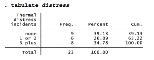
Ordinarily, tabulate displays value labels. The nolabel option reveals that the numeric codes behind these value labels are 0 = “none”, 1 = “1 or 2”, and 2 = “3 plus”.
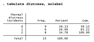
We can use these codes to create a new dummy variable, any, coded 0 for no distress and 1 for one or more distress incidents:
. generate any = distress
. replace any = 1 if distress == 2
. label variable any “Any thermal distress”
To check what these generate and replace commands accomplished, and be sure that missing values were handled correctly, . tabulate distress any, miss

Logistic regression models how a {0,1} dichotomy such as any depends on one or more x variables. The syntax of logit resembles that of regress and most other model-fitting commands, with the dependent variable listed first.
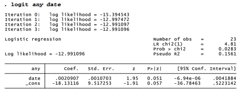
The logit iterative estimation procedure maximizes the log of the likelihood function, shown above the logistic table. At iteration 0, the log likelihood describes the fit of a model including only the constant. The last log likelihood describes the fit of the final model,
L = -18.13116 + .0020907 date [9.1]
where L represents the predicted logit, or log odds, of any distress incidents:
L = ln[P(any = 1) / P(any = 0)] [9.2]
An overall %2 test at the upper right evaluates the null hypothesis that all coefficients in the model, except the constant, equal zero,
![]()
where ln Li ; is the initial or iteration 0 (model with constant only) log likelihood, and ln Lr is the final iteration’s log likelihood. Here,
X2 = -2[-15.394543 – (-12.991096)]
= 4.81
The probability of a greater /2, with 1 degree of freedom (the difference in complexity between initial and final models), is low enough (.0283) to reject the null hypothesis in this example. Consequently, date does have a significant effect.
Less accurate, though convenient, tests are provided by the asymptotic z (standard normal) statistics displayed with logit results. With one predictor variable, that predictor’s z statistic and the overall /2 statistic test equivalent hypotheses, analogous to the usual t and F statistics in simple OLS regression. Unlike their OLS counterparts, the logit z approximation and /2 tests sometimes disagree (they do here). The /2 test has more general validity.
Like some other Stata maximum-likelihood procedures, logit displays a pseudo R2:
![]()
For this example,
pseudo R2 = 1 – (-12.991096) / (-15.394543)
= .1561
Although pseudo R2 statistics provide a quick way to describe or compare the fit of different models for the same dependent variable, they lack the straightforward explained-variance interpretation of true R2 in OLS regression.
After logit, the predict command (with no options) obtains predicted probabilities,
Phat = 1 / (1 + e-L ) [9.5]
Graphed against date, these predicted probabilities follow an S-shaped logistic curve. Because we specified format %td date earlier after we defined variable date, values are appropriately labeled on the horizontal or time axis in Figure 9.1.

The coefficient in this logit example ( .0020907) describes date’s effect on the logit or log odds that any thermal distress incidents occur. Each additional day increases the predicted log odds of thermal distress by .0020907. Equivalently, we could say that each additional day multiplies predicted odds of thermal distress by e 0020907 = 1.0020929; each 100 days therefore multiplies the odds by (e 0020907 ) 100 = 1.23. (e » 2.71828, the base number for natural logarithms.) Stata can make these calculations utilizing the _b[varname] coefficients stored after any estimation:
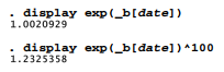
We could also simply include an or (odds ratio) option on the logit command line. A third way to obtain odds ratios employs the logistic command, described in the next section. logistic fits exactly the same model as logit, but its default output table displays odds ratios rather than coefficients.
Source: Hamilton Lawrence C. (2012), Statistics with STATA: Version 12, Cengage Learning; 8th edition.
Dead indited articles, Really enjoyed looking through.