What Are Cycles?

In mathematical terms, the cosine (and sine) function describes a cycle. Figure 19.2 shows a right-angle triangle (one with a 90-degree angle). The side across from the 90-degree angle is the hypotenuse, labeled (H). A cosine of an angle is the ratio of the adjacent side to the hypotenuse. For example, in Figure 19.2, the cosine for angle U is A/H. Thus, for every angle, there is a specific cosine value.

Within a circle (the unit circle), we can create a triangle from each point along the circle perimeter. As demonstrated in Figure 19.3, using the radius length of the circle as the hypotenuse and the length along the
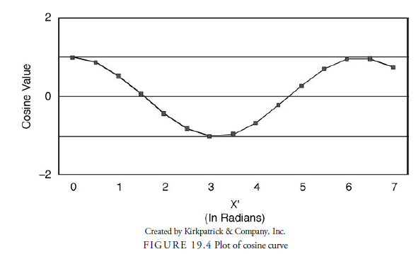
horizontal axis to an intersection perpendicular to the perimeter point, we can calculate the cosine of the angle between each hypotenuse and the axis line for each point along the perimeter. The cosine value is the ratio of the length along the x-axis (X’) divided by the radius of the circle. The cosine value will always be one or less because X can never be larger than the radius. As the point works its way around the circle counterclockwise, we can plot the series of cosine values in another chart with the angle (in radians) along the x-axis and the cosine value along the y-axis, as shown in Figure 19.4. As you can see in the figure, this results in a curve with values oscillating between -1 and 1. This curve is known as a cosine wave and is the basis for calculating the existence of cycles or waves in time series data.

Of course, cycles can have different parameters. They can be long from bottom to bottom, high and short, and begin from different locations. The location along the cycle of each point can be defined by the following formula:

f(x) = a x cos(bx + c) + d
Where: a is the amplitude
bx is the period (constant b times x time in radians)
c is the phase (in radians)
d is the error factor

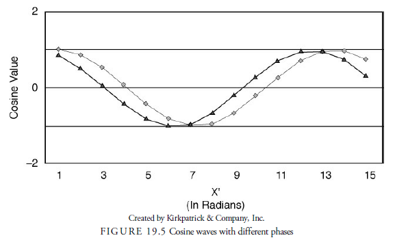
Rather than fully understanding the derivation of cosine waves, it is important to know the specific variables that determine the waveform. Amplitude is the distance from the horizontal axis to the extreme peak or trough. In Figure 19.4, amplitude is 1. An amplitude of 2 would result in a cosine wave twice the height of the cosine waves with an amplitude of 1. Period is the distance between consecutive lows or consecutive highs. In our usage, the period is the time along the horizontal axis that it takes for the cycle to return to its original position. Figure 19.5 shows two cosine waves with different phases. Phase determines how far from the y-axis the particular cycle begins. It thus determines the offset between two cycles of different phases.

If we know the parameter constants for each variable, we can plot any cosine wave. If there are multiple cosine waves, we can calculate each and add them together in what is called summation. James Hurst more thoroughly developed this idea in his book The Profit Magic of Stock Transaction Timing (1970). The presumption in markets is that there is no one specific cycle but many cycles that, when summed, form the plot of prices. The forecasting problem then is to reverse the process and go from the price plot to the cosine formula to determine how many cosine waves and their parameters exist in the data. From this knowledge, presumably the direction of prices can be foretold by extrapolating the waves into the future.

Like all theories related to the markets, the theory of cycles is logical but impossible to quantify, at least with the present level of mathematics. Many methods have been invented to recognize waves in time series data, but none has been able to duplicate market price sequences with reliable accuracy. There are many reasons for this, the primary one being that the parameters in the cosine functions of market prices are not constants. Hurst calls this the principle of variation. Amplitude and period, for example, vary over time. Most mathematical means of determining cosines from time series data assume that the parameters are constants. This does not mean that the standard methods of analysis of time series are useless, however. The changes in parameters appear to take place slowly rather than suddenly. By analyzing prices through conventional cosine analysis over specific but different periods, we can see how the parameters change. Amplitude appears to change quickly at times, but period appears to change more slowly. Thus, if we can at least estimate the period with some degree of accuracy, as analysts, we have a useful indicator. We cannot predict future price levels, but with an estimate of period, we can potentially predict the timing of future highs and lows.

Other Aspects of Cycle Analysis

There are several other aspects of cycle analysis of which the technical analyst needs to be aware. Accuracy concerns exist because cycle periods are indefinite and have error. Cycle translations and inversions make cycle analysis more difficult. However, due to harmonic properties, determining one cycle period often leads the analyst to determining cycle periods that are multiples of that initial cycle.

Accuracy

Just because the analysis of financial time series data may suggest cycles exist does not imply that the cycles are precise. As mentioned earlier, all three aspects of a wave vary over time, and as wave is added to wave, the errors become large. Because market cycles tend to synchronize at lows, the estimate of the phase is relatively easy. The analysis just begins at a major price low where presumably most cycle lows coincide. The estimate of amplitude varies too much for projection purposes. Amplitude is often called the power of the cycle in electronic analysis circles, where it tends to be a constant in those applications. In the financial world, power can be influenced greatly by exogenous, unpredictable events. The study of amplitude becomes nonproductive. The third aspect of the cosine wave, the period, often remains relatively constant but can sometime have large errors. Estimates are based on immediate past price history. As an example, a 20-day cycle low can occur several days before or after the expected 20 days from the last low, which itself may have been several days before or after its ideal location. The 20-day cycle, from spectral or other analysis, may only be 19.2 days, or it may be 20.4 days. Cycle periods, therefore, are indefinite and have error. This means that for investment purposes, all cycles should be used only as a guide. Even the well-established, seasonal cycle has actual high and low dates that vary considerably from year to year.

Harmonics

One of the interesting aspects of cycles first observed by Hurst in market data is that cycles tend to have period lengths a multiple of two or three longer or shorter than the next larger or smaller cycles. In other words, a cycle of 20 days will indicate that another longer cycle of either 40- or 60-days length exists and that another shorter cycle of 7 or 10 days exists. The longer is either two times or three times the observed cycle, and the shorter is either 1/3 or 1/2 the observed cycle. This observation is useful when one specific cycle is determined because it leads the analyst to what intervals to look for in longer and shorter cycles. Hurst believed that the ratio of two is more common. Others, such as Tony Plummer (2003), have hypothesized that three is the correct multiple.

In the April 1987 issue of Technical Analysis of Stocks and Commodities Magazine, Frank Tarkany compared his analysis of weekly market cycles with that of three other well-known analysts. Table 19.1 provides a summary of Tarkany’s comparisons. All four of the analysts found 26-week cycles; this 26-week cycle is the base cycle. These analysts also noticed multiples of 26 weeks, suggesting that an autocorrelation exists between cycle periods. These cycle periods are called nominal periods because they occur regularly in most financial time series data.

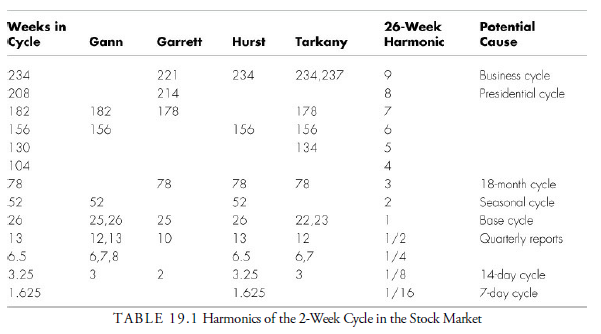
Notice that several of the cycles appearing in Table 19.1 are stock market cycles we have mentioned in previous chapters. The well-known presidential cycle is very dependable, as is the seasonal cycle. They are both multiples of the 26-week base cycle—the seasonal cycle by two, and the presidential cycle by eight (or 2 x 2 x 2). Thus, the Hurst hypothesis that cycles tend to occur in multiples of two or three seems to make sense.

Inversions

One of the most difficult observations for the analyst to face is the inversion. Occasionally, where a cycle low is expected, a peak occurs instead. No satisfactory explanation has been given for its existence, but several observations have been noted.

Inversions can occur at either peaks or troughs, but most often they occur at peaks in harmonic cycles when the next longer cycle is at a peak. This make sense only if the next higher order cycle is a multiple of two. For example, a cycle of 20 days should make a low every 20 days. If the next higher order cycle is 40 days, synchronous with the 20-day cycle, and peaking, a 40-day peak ideally should occur just as a 20-day cycle is making a low. Thus, the 20-day cycle low is masked by the peaking of the 40-day cycle and is often difficult to decipher. When this occurs, the inverted cycle low often has just a small short-term “dip” within the peak of the higher order cycle. This dip resembles an M where the small low between the two small peaks is the actual cycle low that is being overcome by the longer cycle. Proof of the low coinciding with the longer-cycle high occurs when the subsequent decline breaks below the dip. If a longer cycle is due to peak, this is the sign that its declining portion has begun.

Previously, we noted that cycles are not strict harmonics but specific time-separated events. The habit of producing lows at constant intervals can be interspersed with highs at the same intervals because both are important market events. Thus, a long string of events occurring at specific intervals that is primarily dominated by low events but interspersed with occasional high events at the same periodic times can look like a harmonic wave for the period that the lows are occurring but be confusing from a cyclical standpoint. However, the progression is only a time sequence of events. Analysts thus assume inversions are anomalies within a harmonic-type wave when the wave is actually an event wave, not a true mathematically defined cycle.

Source: Kirkpatrick II Charles D., Dahlquist Julie R. (2015), Technical Analysis: The Complete Resource for Financial Market Technicians, FT Press; 3rd edition.