How Is a Simple Moving Average Calculated?

Table 14.1 contains the daily closing prices for WMT (Walmart) from November 18, 2014 through February 26, 2015. Most moving averages of prices are based on closing prices, but they can be calculated on highs, lows, daily means, or any other value as long as the price type is consistent throughout the calculations. We use closing prices.

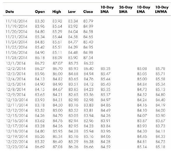
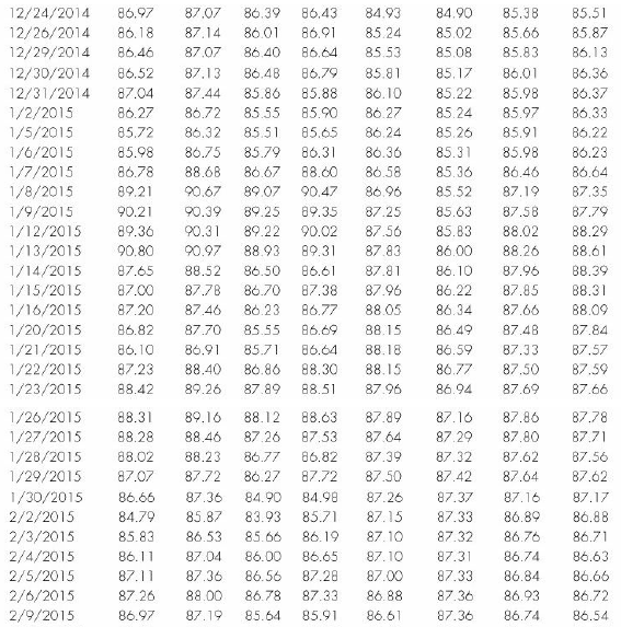
The most commonly used type of moving average is the simple moving average (SMA), sometimes referred to as an arithmetic moving average. An SMA is constructed by adding a set of data and then dividing by the number of observations in the period being examined. For example, look at the ten-day SMA in Table 14.1. We begin by summing the closing prices for the first ten days. We then divide this sum by 10 to give us the mean price for that ten-day period. Thus, on the tenth day, the ten-day simple moving average would be the mean closing price for WMT for Days 1 through 10, or $85.35.

On Day 11, the moving average changes. To calculate the moving average for Day 11, we calculate the mean price for Days 2 through 11. In other words, the closing price for Day 1 is dropped from the data set, whereas the price for Day 11 is added. The formula for calculating a ten-day simple moving average is as follows:

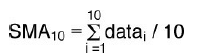
Of course, we can construct moving averages of different lengths. In Table 14.1, you can also see a 26-day moving average. This SMA is simply calculated by adding the 26 most recent closing prices and dividing by 26.

Although a moving average can smooth prices over any desired period, some of the more popular daily moving averages are for the periods 200, 60, 50, 30, 20, and 10 days. These periods are somewhat arbitrary and were chosen in the days before computers when the calculations had to be done by hand or on a crank adding machine. Gartley (1935), for example, used the 200-day moving average in his work. Simply, numbers divisible by 10 were easier to calculate. Also, the 10-day, 20-day, and 60-day moving averages summarize approximately two weeks, one month, and three months (one fiscal quarter) of trading data, respectively.

Once calculated, moving averages are plotted on a price chart. Figure 14.1 shows a plot of the 26-day simple moving average for WMT. From early November through late January, the moving average is an upward sloping curve, indicating an upward trend in Walmart’s price. The daily fluctuations are smoothed by the moving average so that the analyst can see the underlying trend without being distracted by the small, daily movements.

A rising moving average indicates an upward trend, whereas a falling moving average indicates a downward trend. Although the moving average helps us discern a trend, it does so after the trend has begun. Thus, the moving average is a lagging indicator. By definition, the moving average is an indicator that is based on past prices. For example, Figure 14.1 shows an upward trend in WMT prices beginning in late October. However, an upward movement in the SMA does not occur until approximately early November. Remember that according to technical analysis principles, we want to be trading with the trend. Using a moving average will always give us some delay in signaling a change in trend.

1. Length of Moving Average

Because moving averages can be calculated for various lengths of time, which length is best to use? Of course, a longer time period includes more data observations, and, thus, more information. By including more data in the calculation of the moving average, each day’s data becomes relatively less important in the calculation. Therefore, a large change in the value on one day does not have a large impact on the longer moving average. This can be an advantage if this large change is a one-day, irregular outlier in the data.

However, if this large move represents the beginning of a significant change in the trend, it takes longer for the underlying trend change to be discernable. Thus, the longer moving average is slower to pick up trend changes but less likely to falsely indicate a trend change due to a short-term blip in the data.

Figure 14.2, for example, shows both a 13-day and a 26-day SMA plotted for WMT. Notice how the shorter, 13-day moving average shows more variability than the longer, 26-day moving average. The 26-day moving average is said to be the “slower” moving average. Although it provides more smoothing, the 26-day smoothing average is also slower at signaling underlying trend changes. Notice the 13-day SMA troughs in late October/early November, signaling a change in trend; a week later, the slower, 26-day SMA is flat but and gradually turning upward. Thus, the 26-day SMA is slower to indicate a trend change.

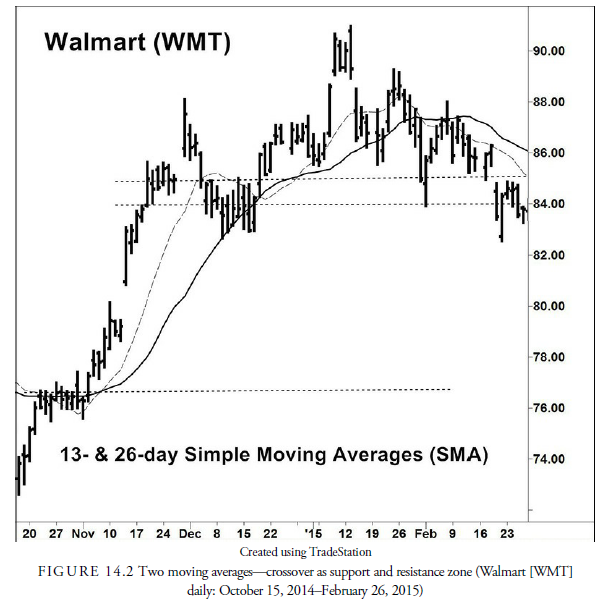
Because spotting a trend reversal as soon as possible maximizes trading profits, the 13-day SMA may first appear to give superior information; however, remember that the faster SMA has a disadvantage of potentially giving a false signal of a changing trend direction. For example, look at early December in Figure 14.2. The 13-day SMA flattens out, suggesting an end to the upward price trend. After the fact, however, we can see that a trend reversal did not occur until mid-January. The 13-day SMA was overly sensitive to a temporary decrease in price. During this period, the slower 26-day SMA continued to signal correctly an upward trend.

2. Using Multiple Moving Averages

Analysis is not limited to the information provided by a single moving average. Considering various moving averages of various lengths simultaneously can increase the analysts’ information set. For example, as shown in Figure 14.2, a support or resistance level often occurs where two moving averages cross. Where the shorter moving average crosses above the longer is often taken as a mechanical buy signal, or at least a sign that the price trend is upward. Likewise, it is considered a sell signal when the shorter declines below the longer. Many successful moving average strategies use moving averages as the principal determinant of trend and then use shorter-term moving averages either as trailing stops or as signals. In some instances, moving averages are used to determine trend, and then chart patterns are used as entry and exit signals.

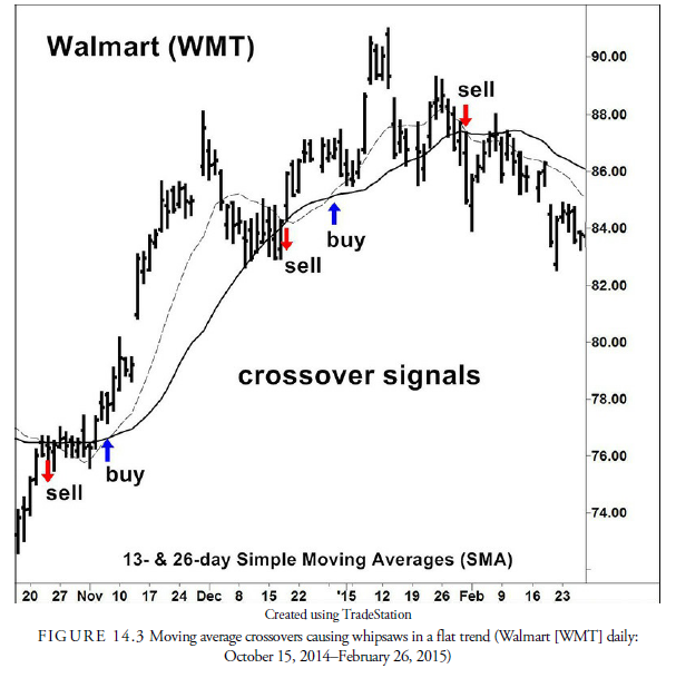
Using these types of dual moving average signals during a sideways trend in prices, however, can result in a number of whipsaws. This problem can be seen in Figure 14.3. This is essentially the same problem that occurs during the standard sideways trend in a congestion area. It is difficult to determine from such action in which way prices are going to break out. Meanwhile, they oscillate back and forth within the support and resistance levels. A moving average provides no additional information on which way the trend will eventually break. Indeed, a moving average requires a trend for a crossover to be profitable. This means that the analyst must be sure that a trend exists before using moving average crossovers for signals. Otherwise—and some traders are willing to take the risk of short-term whipsaws so they don’t miss the major trend—a plurality of signals will be incorrect and produce small losses while waiting for the one signal that will produce the large profit. This can be a highly profitable method provided the analyst has the stomach and discipline to continue with the small losses, and it often is the basis for many long-term trend systems. It also demonstrates how, with proper discipline, one can profit while still losing on a majority of small trades.

Source: Kirkpatrick II Charles D., Dahlquist Julie R. (2015), Technical Analysis: The Complete Resource for Financial Market Technicians, FT Press; 3rd edition.