Production with One Variable Input (Labor)

When deciding how much of a particular input to buy, a firm has to compare the benefit that will result with the cost of that input. Sometimes it is useful to look at the benefit and the cost on an incremental basis by focusing on the additional out- put that results from an incremental addition to an input. In other situations, it is useful to make the comparison on an average basis by considering the result of substantially increasing an input. We will look at benefits and costs in both ways.

When capital is fixed but labor is variable, the only way the firm can produce more output is by increasing its labor input. Imagine, for example, that you are managing a clothing factory. Although you have a fixed amount of equipment, you can hire more or less labor to sew and to run the machines. You must decide how much labor to hire and how much clothing to produce. To make the deci- sion, you will need to know how the amount of output q increases (if at all) as the input of labor L increases.

Table 6.1 gives this information. The first three columns show the amount of output that can be produced in one month with different amounts of labor and capital fixed at 10 units. The first column shows the amount of labor, the second the fixed amount of capital, and the third total output. When labor input is zero, output is also zero. Output then increases as labor is increased up to an input of 8 units. Beyond that point, total output declines: Although initially each unit of labor can take greater and greater advantage of the existing machinery and plant, after a certain point, additional labor is no longer useful and indeed can be counterproductive. Five people can run an assembly line better than two, but ten people may get in one another ’s way.

1. Average and Marginal Products

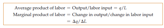
The contribution that labor makes to the production process can be described on both an average and a marginal (i.e.,incremental) basis. The fourth column in Table 6.1 shows the average product of labor (APL ), which is the output per unit of labor input. The average product is calculated by dividing the total out­put q by the total input of labor L. The average product of labor measures the productivity of the firm’s workforce in terms of how much output each worker produces on average. In our example, the average product increases initially but falls when the labor input becomes greater than four.

The fifth column of Table 6.1 shows the marginal product of labor (MP_L). This • marginal product is the additional output produced as the labor input is increased by 1 unit. For -Additional output produced as example, with capital fixed at 10 units, when the labor input increases from 2 to ^{an input is increased by one unit} 3, total output increases from 30 to 60, creating an additional output of 30 (i.e.,

60-30) units. The marginal product of labor can be written as Aq/AL—in other words, the change in output Aq resulting from a 1-unit increase in labor input AL.

Remember that the marginal product of labor depends on the amount of capital used. If the capital input increased from 10 to 20, the marginal product of labor most likely would increase. Why? Because additional workers are likely to be more productive if they have more capital to use. Like the average product, the marginal product first increases then falls—in this case, after the third unit of labor.

To summarize:

2. The Slopes of the Product Curve

Figure 6.1 plots the information contained in Table 6.1. (We have connected all the points in the figure with solid lines.) Figure 6.1 (a) shows that as labor is increased, output increases until it reaches the maximum output of 112; thereaf- ter, it falls. The portion of the total output curve that is declining is drawn with a dashed line to denote that producing with more than eight workers is not economically rational; it can never be profitable to use additional amounts of a costly input to produce less output.

Figure 6.1 (b) shows the average and marginal product curves. (The units on the vertical axis have changed from output per month to output per worker per month.) Note that the marginal product is positive as long as output is increas- ing, but becomes negative when output is decreasing.

It is no coincidence that the marginal product curve crosses the horizontal axis of the graph at the point of maximum total product. This happens because adding a worker in a manner that slows production and decreases total output implies a negative marginal product for that worker.

The average product and marginal product curves are closely related. When the marginal product is greater than the average product, the average product is increas- ing. This is the case for labor inputs up to 4 in Figure 6.1 (b). If the output of an additional worker is greater than the average output of each existing worker (i.e., the marginal product is greater than the average product), then adding the worker causes average output to rise. In Table 6.1, two workers produce 30 units of output, for an average product of 15 units per worker. Adding a third worker increases output by 30 units (to 60), which raises the average product from 15 to 20.

Similarly, when the marginal product is less than the average product, the average product is decreasing. This is the case when the labor input is greater than 4 in Figure 6.1 (b). In Table 6.1, six workers produce 108 units of output, for an aver- age product of 18. Adding a seventh worker contributes a marginal product of only 4 units (less than the average product), reducing the average product to 16.

We have seen that the marginal product is above the average product when the average product is increasing and below the average product when the aver- age product is decreasing. It follows, therefore, that the marginal product must equal the average product when the average product reaches its maximum. This happens at point E in Figure 6.1 (b).

Why, in practice, should we expect the marginal product curve to rise and then fall? Think of a television assembly plant. Fewer than ten workers might be insufficient to operate the assembly line at all. Ten to fifteen workers might be able to run the assembly line, but not very efficiently. If adding a few more workers allowed the assembly line to operate much more efficiently, the mar- ginal product of those workers would be very high. This added efficiency, however, might start to diminish once there were more than 20 workers. The marginal product of the twenty-second worker, for example, might still be very high (and above the average product), but not as high as the marginal product of the nineteenth or twentieth worker. The marginal product of the twenty-fifth worker might be lower still, perhaps equal to the average product. With 30 workers, adding one more worker would yield more output, but not very much more (so that the marginal product, while positive, would be below the average product). Once there were more than 40 workers, additional workers would simply get in each other ’s way and actually reduce output (so that the marginal product would be negative).

3. The Average Product of Labor Curve

The geometric relationship between the total product and the average and marginal product curves is shown in Figure 6.1 (a). The average product of labor is the total product divided by the quantity of labor input. At B, for example, the average prod- uct is equal to the output of 60 divided by the input of 3, or 20 units of output per unit of labor input. This ratio, however, is exactly the slope of the line running from the origin to B in Figure 6.1 (a). In general, the average product of labor is given by the slope of the line drawn from the origin to the corresponding point on the total product curve.

4. The Marginal Product of Labor Curve

As we have seen, the marginal product of labor is the change in the total product resulting from an increase of one unit of labor. At A, for example, the marginal product is 20 because the tangent to the total product curve has a slope of 20. In general, the marginal product of labor at a point is given by the slope of the total prod- uct at that point. We can see in Figure 6.1 (b) that the marginal product of labor increases initially, peaks at an input of 3, and then declines as we move up the total product curve to C and D. At D, when total output is maximized, the slope of the tangent to the total product curve is 0, as is the marginal product. Beyond that point, the marginal product becomes negative.

THE RELATIONSHIP BETWEEN THE AVERAGE AND  MARGINAL PRODUCTS Note the graphical relationship between average and marginal products in Figure 6.1 (a). At B, the marginal product of labor (the slope of the tangent to the total product curve at B—not shown explicitly) is greater than the average product (dashed line 0B). As a result, the average product of labor increases as we move from B to C. At C, the average and marginal products of labor are equal: While the average product is the slope of the line from the origin,

0C, the marginal product is the tangent to the total product curve at C (note the equality of the average and marginal products at point E in Figure 6.1 (b)). Finally, as we move beyond C toward D, the marginal product falls below the average product; you can check that the slope of the tangent to the total product curve at any point between C and D is lower than the slope of the line from the origin.

5. The Law of Diminishing Marginal Returns

A diminishing marginal product of labor (as well as a diminishing marginal product of other inputs) holds for most production processes. The law of dimin- ishing marginal returns states that as the use of an input increases in equal increments (with other inputs fixed), a point will eventually be reached at which the resulting additions to output decrease. When the labor input is small (and capital is fixed), extra labor adds considerably to output, often because workers are allowed to devote themselves to specialized tasks. Eventually, however, the law of diminishing marginal returns applies: When there are too many workers, some workers become ineffective and the marginal product of labor falls.

The law of diminishing marginal returns usually applies to the short run when at least one input is fixed. However, it can also apply to the long run.

Even though inputs are variable in the long run, a manager may still want to analyze production choices for which one or more inputs are unchanged. Suppose, for example, that only two plant sizes are feasible and that management must decide which to build. In that case, management would want to know when diminishing marginal returns will set in for each of the two options.

Do not confuse the law of diminishing marginal returns with possible changes in the quality of labor as labor inputs are increased (as would likely occur, for example, if the most highly qualified laborers are hired first and the least qualified last). In our analysis of production, we have assumed that all labor inputs are of equal quality; diminishing marginal returns results from lim- itations on the use of other fixed inputs (e.g., machinery), not from declines in worker quality. In addition, do not confuse diminishing marginal returns with negative returns. The law of diminishing marginal returns describes a declining marginal product but not necessarily a negative one.

The law of diminishing marginal returns applies to a given production tech- nology. Over time, however, inventions and other improvements in technology may allow the entire total product curve in Figure 6.1 (a) to shift upward, so that more output can be produced with the same inputs. Figure 6.2 illustrates this principle. Initially the output curve is given by O1, but improvements in tech- nology may allow the curve to shift upward, first to O2, and later to O3.

Suppose, for example, that over time, as labor is increased in agricultural production, technological improvements are being made. These improvements might include genetically engineered pest-resistant seeds, more powerful and effective fertilizers, and better farm equipment. As a result, output changes from A (with an input of 6 on curve O1) to B (with an input of 7 on curve O2) to C (with an input of 8 on curve O3).

The move from A to B to C relates an increase in labor input to an increase in output and makes it appear that there are no diminishing marginal returns when in fact there are. Indeed, the shifting of the total product curve suggests that there may be no negative long-run implications for economic growth. In fact, as

we can see in Example 6.1, the failure to account for long-run improvements in technology led British economist Thomas Malthus wrongly to predict dire con- sequences from continued population growth.

Source: Pindyck Robert, Rubinfeld Daniel (2012), Microeconomics, Pearson, 8th edition.