Our analysis of input substitution in the production process has shown us what happens when a firm substitutes one input for another while keeping output constant. However, in the long run, with all inputs variable, the firm must also consider the best way to increase output. One way to do so is to change the scale of the operation by increasing all of the inputs to production in proportion. If it takes one farmer working with one harvesting machine on one acre of land to produce 100 bushels of wheat, what will happen to output if we put two farmers to work with two machines on two acres of land? Output will almost certainly increase, but will it double, more than double, or less than double? Returns to scale is the rate at which output increases as inputs are increased proportion- ately. We will examine three different cases: increasing, constant, and decreasing returns to scale.
INCREASING RETURNS TO SCALE If output more than doubles when inputs are doubled, there are increasing returns to scale. This might arise because the larger scale of operation allows managers and workers to specialize in their tasks and to make use of more sophisticated, large-scale factories and equipment. The automobile assembly line is a famous example of increasing returns.
The prospect of increasing returns to scale is an important issue from a public- policy perspective. If there are increasing returns, then it is economically advan- tageous to have one large firm producing (at relatively low cost) rather than to have many small firms (at relatively high cost). Because this large firm can control the price that it sets, it may need to be regulated. For example, increasing returns in the provision of electricity is one reason why we have large, regulated power companies.
CONSTANT RETURNS TO SCALE A second possibility with respect to the scale of production is that output may double when inputs are doubled. In this case, we say there are constant returns to scale. With constant returns to scale, the size of the firm’s operation does not affect the productivity of its factors: Because one plant using a particular production process can easily be repli- cated, two plants produce twice as much output. For example, a large travel agency might provide the same service per client and use the same ratio of capital (office space) and labor (travel agents) as a small agency that services fewer clients.
DECREASING RETURNS TO SCALE Finally, output may less than double when all inputs double. This case of decreasing returns to scale applies to some firms with large-scale operations. Eventually, difficulties in organizing and run- ning a large-scale operation may lead to decreased productivity of both labor and capital. Communication between workers and managers can become dif- ficult to monitor as the workplace becomes more impersonal. Thus, the decreas- ing-returns case is likely to be associated with the problems of coordinating tasks and maintaining a useful line of communication between management and workers.
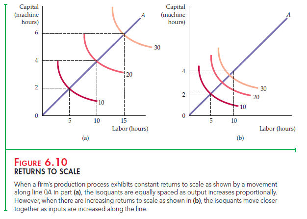
When a firm’s production process exhibits constant returns to scale as shown by a movement along line 0A in part (a), the isoquants are equally spaced as output increases proportionally. However, when there are increasing returns to scale as shown in (b), the isoquants move closer together as inputs are increased along the line.
Describing Returns to Scale
Returns to scale need not be uniform across all possible levels of output. For example, at lower levels of output, the firm could have increasing returns to scale, but constant and eventually decreasing returns at higher levels of output.
The presence or absence of returns to scale is seen graphically in the two parts of Figure 6.10. The line 0A from the origin in each panel describes a production pro- cess in which labor and capital are used as inputs to produce various levels of out- put in the ratio of 5 hours of labor to 2 hours of machine time. In Figure 6.10 (a), the firm’s production function exhibits constant returns to scale. When 5 hours of labor and 2 hours of machine time are used, an output of 10 units is produced. When both inputs double, output doubles from 10 to 20 units; when both inputs triple, output triples, from 10 to 30 units. Put differently, twice as much of both inputs is needed to produce 20 units, and three times as much is needed to produce 30 units.
In Figure 6.10 (b), the firm’s production function exhibits increasing returns to scale. Now the isoquants come closer together as we move away from the origin along 0A. As a result, less than twice the amount of both inputs is needed to increase production from 10 units to 20; substantially less than three times the inputs are needed to produce 30 units. The reverse would be true if the pro- duction function exhibited decreasing returns to scale (not shown here). With decreasing returns, the isoquants are increasingly distant from one another as output levels increase proportionally.
Returns to scale vary considerably across firms and industries. Other things being equal, the greater the returns to scale, the larger the firms in an industry are likely to be. Because manufacturing involves large investments in capital equip- ment, manufacturing industries are more likely to have increasing returns to scale than service-oriented industries. Services are more labor-intensive and can usually be provided as efficiently in small quantities as they can on a large scale.
Source: Pindyck Robert, Rubinfeld Daniel (2012), Microeconomics, Pearson, 8th edition.
You are my aspiration, I own few blogs and very sporadically run out from to brand.