Price Supports and Production Quotas

Besides imposing a minimum price, the government can increase the price of a good in other ways. Much of American agricultural policy is based on a system of price supports, whereby the government sets the market price of a good above the free-market level and buys up whatever output is needed to maintain that price. The government can also increase prices by restricting production, either directly or through incentives to producers. In this section, we show how these policies work and examine their impact on consumers, producers, and the federal budget.

1. Price Supports

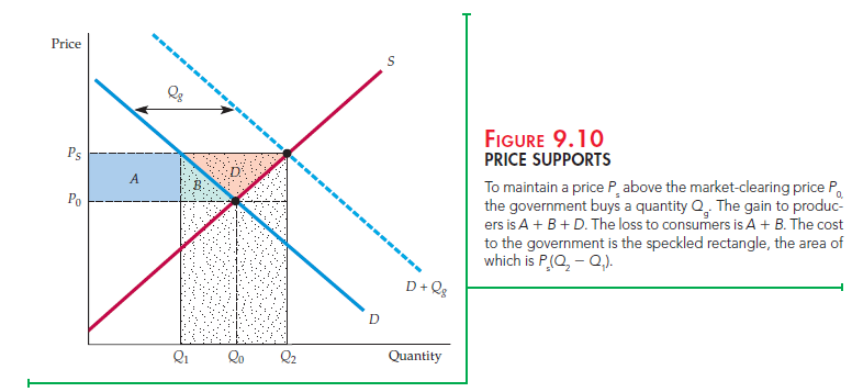
In the United States, price supports aim to increase the prices of dairy prod- ucts, tobacco, corn, peanuts, and so on, so that the producers of those goods can receive higher incomes. Under a price support program, the government sets a support price Ps and then buys up whatever output is needed to keep the market price at this level. Figure 9.10 illustrates this. Let’s examine the resulting gains and losses to consumers, producers, and the government.

CONSUMERS At price Ps, the quantity that consumers demand falls to Q1, but the quantity supplied increases to Q2. To maintain this price and avoid hav- ing inventories pile up in producer warehouses, the government must buy the quantity Qg = Q2 − Q1. In effect, because the government adds its demand Qg to the demand of consumers, producers can sell all they want at price Ps.

Because those consumers who purchase the good must pay the higher price Ps instead of Po, they suffer a loss of consumer surplus given by rectangle A. Because of the higher price, other consumers no longer buy the good or buy less of it, and their loss of surplus is given by triangle B. So, as with the minimum price that we examined above, consumers lose, in this case by an amount

PRODUCERS On the other hand, producers gain (which is why such a policy is implemented). Producers are now selling a larger quantity Q₂ instead of Q₀, and at a higher price P_s. Observe from Figure 9.10 that producer surplus increases by the amount

THE GOVERNMENT But there is also a cost to the government (which must be paid for by taxes, and so is ultimately a cost to consumers). That cost is (Q₂ – Q₁)P_s, which is what the government must pay for the output it purchases. In Figure 9.10, this amount is represented by the large speckled rectangle. This cost may be reduced if the government can “dump” some of its purchases—i.e., sell them abroad at a low price. Doing so, however, hurts the ability of domes­tic producers to sell in foreign markets, and it is domestic producers that the government is trying to please in the first place.

What is the total welfare cost of this policy? To find out, we add the change in consumer surplus to the change in producer surplus and then subtract the cost to the government. Thus the total change in welfare is

In terms of Figure 9.10, society as a whole is worse off by an amount given by the large speckled rectangle, less triangle D.

As we will see in Example 9.4, this welfare loss can be very large. But the most unfortunate part of this policy is the fact that there is a much more efficient way to help farmers. If the objective is to give farmers an additional income equal to A + B + D, it is far less costly to society to give them this money directly rather than via price supports. Because price supports are costing consumers A + B anyway, by paying farmers directly, society saves the large speckled rectangle, less triangle D. So why doesn’t the government simply give farmers money? Perhaps because price supports are a less obvious giveaway and, therefore, politically more attractive.8

2. Production Quotas

Besides entering the market and buying up output—thereby increasing total demand—the government can also cause the price of a good to rise by reducing supply. It can do this by decree—that is, by simply setting quotas on how much each firm can produce. With appropriate quotas, the price can then be forced up to any arbitrary level.

As we will see in Example 9.5, this is how many city governments main- tain high taxi fares. They limit total supply by requiring each taxicab to have a medallion, and then limit the total number of medallions. Another example is the control of liquor licenses by state governments. By requiring any bar or res- taurant that serves alcohol to have a liquor license and then limiting the number of licenses, entry by new restaurateurs is limited, which allows those who have licenses to earn higher prices and profit margins.

The welfare effects of production quotas are shown in Figure 9.11. The government restricts the quantity supplied to Q1, rather than the market- clearing level Q0. Thus the supply curve becomes the vertical line S’ at Q1. Consumer surplus is reduced by rectangle A (those consumers who buy the good pay a higher price) plus triangle B (at this higher price, some consum- ers no longer purchase the good). Producers gain rectangle A (by selling at a higher price) but lose triangle C (because they now produce and sell Q1 rather than Q0). Once again, there is a deadweight loss, given by triangles B and C.

INCENTIVE PROGRAMS In U.S. agricultural policy, output is reduced by incentives rather than by outright quotas. Acreage limitation programs give farmers financial incentives to leave some of their acreage idle. Figure 9.11 also shows the welfare effects of reducing supply in this way. Note that because farmers agree to limit planted acreage, the supply curve again becomes completely inelastic at the quantity Q1, and the market price is increased from P0  to Ps.

As with direct production quotas, the change in consumer surplus is

Farmers now receive a higher price for the production Q₁, which corresponds to a gain in surplus of rectangle A. But because production is reduced from Q₀ to Q₁, there is a loss of producer surplus corresponding to triangle C. Finally, farmers receive money from the government as an incentive to reduce produc­tion. Thus the total change in producer surplus is now

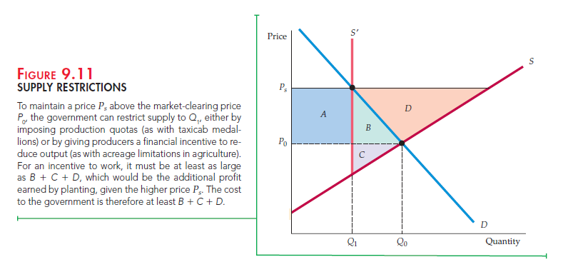
The cost to the government is a payment sufficient to give farmers an incen- tive to reduce output to Q1. That incentive must be at least as large as B + C + D because that area represents the additional profit that could be made by plant- ing, given the higher price Ps. (Remember that the higher price Ps  gives farmers an incentive to produce more even though the government is trying to get them to produce less.) Thus the cost to the government is at least B + C + D, and the total change in producer surplus is

This is the same change in producer surplus as with price supports main­tained by government purchases of output. (Refer to Figure 9.10.) Farmers, then, should be indifferent between the two policies because they end up gaining the same amount of money from each. Likewise, consumers lose the same amount of money.

Which policy costs the government more? The answer depends on whether the sum of triangles B + C + D in Figure 9.11 is larger or smaller than (Q₂ – Q₁)P_s (the large speckled rectangle) in Figure 9.10. Usually it will be smaller, so that an acreage-limitation program costs the government (and society) less than price supports maintained by government purchases.

Still, even an acreage-limitation program is more costly to society than simply handing the farmers money. The total change in welfare (ACS + APS — Cost to Govt.) under the acreage-limitation program is

Society would clearly be better off in efficiency terms if the government simply gave the farmers A + B + D, leaving price and output alone. Farmers would then gain A + B + D and the government would lose A + B + D, for a total welfare change of zero, instead of a loss of B + C. However, economic efficiency is not always the objective of government policy.

Source: Pindyck Robert, Rubinfeld Daniel (2012), Microeconomics, Pearson, 8th edition.