Production with Two Variable Inputs

We have completed our analysis of the short-run production function in which one input, labor, is variable, and the other, capital, is fixed. Now we turn to the long run, for which both labor and capital are variable. The firm can now pro- duce its output in a variety of ways by combining different amounts of labor and capital. In this section, we will see how a firm can choose among combi- nations of labor and capital that generate the same output. In the first subsec- tion, we will examine the scale of the production process, analyzing how output changes as input combinations are doubled, tripled, and so on.

1. Isoquants

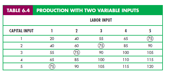
Let’s begin by examining the production technology of a firm that uses two inputs and can vary both of them. Suppose that the inputs are labor and capital and that they are used to produce food. Table 6.4 tabulates the output achievable for various combinations of inputs.

Labor inputs are listed across the top row, capital inputs down the column on the left. Each entry in the table is the maximum (technically efficient) output that can be produced each year with each combination of labor and capital used over that year. For example, 4 units of labor per year and 2 units of capital per year yield 85 units of food per year. Reading along each row, we see that out- put increases as labor inputs are increased, while capital inputs remain fixed. Reading down each column, we see that output also increases as capital inputs are increased, while labor inputs remain fixed.

The information in Table 6.4 can also be represented graphically using iso- quants. An isoquant is a curve that shows all the possible combinations of inputs that yield the same output. Figure 6.5 shows three isoquants. (Each axis in the figure mea- sures the quantity of inputs.) These isoquants are based on the data in Table 6.4, but are drawn as smooth curves to allow for the use of fractional amounts of inputs.

For example, isoquant q1 shows all combinations of labor and capital per year that together yield 55 units of output per year. Two of these points, A and D, cor- respond to Table 6.4. At A, 1 unit of labor and 3 units of capital yield 55 units of output; at D, the same output is produced from 3 units of labor and 1 unit of capi- tal. Isoquant q2 shows all combinations of inputs that yield 75 units of output and corresponds to the four combinations of labor and capital circled in the table (e.g., at B, where 2 units of labor and 3 units of capital are combined). Isoquant q2  lies above and to the right of q1  because obtaining a higher level of output requires

more labor and capital. Finally, isoquant q3 shows labor-capital combinations that yield 90 units of output. Point C, for example, involves 3 units of labor and 3 units of capital, whereas Point E involves 2 units of labor and 5 units of capital.

ISOQUANT MAPS When a number of isoquants are combined in a single graph, we call the graph an isoquant map. Figure 6.5 shows three of the many isoquants that make up an isoquant map. An isoquant map is another way of describing a production function, just as an indifference map is a way of describ- ing a utility function. Each isoquant corresponds to a different level of output, and the level of output increases as we move up and to the right in the figure.

2. Input Flexibility

Isoquants show the flexibility that firms have when making production deci- sions: They can usually obtain a particular output by substituting one input for another. It is important for managers to understand the nature of this flexibil- ity. For example, fast-food restaurants have recently faced shortages of young, low-wage employees. Companies have responded by automating—adding self- service salad bars and introducing more sophisticated cooking equipment. They have also recruited older people to fill positions. As we will see in Chapters 7 and 8, by taking into account this flexibility in the production process, managers can choose input combinations that minimize cost and maximize profit.

3. Diminishing Marginal Returns

Even though both labor and capital are variable in the long run, it is useful for a firm that is choosing the optimal mix of inputs to ask what happens to output as each input is increased, with the other input held fixed. The outcome of this exer- cise is described in Figure 6.5, which reflects diminishing marginal returns to both labor and capital. We can see why there are diminishing marginal returns to labor by drawing a horizontal line at a particular level of capital—say, 3. Reading the levels of output from each isoquant as labor is increased, we note that each additional unit of labor generates less and less additional output. For example, when labor is increased from 1 unit to 2 (from A to B), output increases by 20 (from 55 to 75). However, when labor is increased by an additional unit (from B to C), output increases by only 15 (from 75 to 90). Thus there are diminishing marginal returns to labor both in the long and short run. Because adding one fac- tor while holding the other factor constant eventually leads to lower and lower incremental output, the isoquant must become steeper as more capital is added in place of labor and flatter when labor is added in place of capital.

There are also diminishing marginal returns to capital. With labor fixed, the mar- ginal product of capital decreases as capital is increased. For example, when capital is increased from 1 to 2 and labor is held constant at 3, the marginal product of capi- tal is initially 20 (75 – 55) but falls to 15 (90 – 75) when capital is increased from 2 to 3.

4. Substitution Among Inputs

With two inputs that can be varied, a manager will want to consider substituting one input for another. The slope of each isoquant indicates how the quantity of one input can be traded off against the quantity of the other, while output is held constant. When the negative sign is removed, we call the slope the marginal rate of technical substitution (MRTS). The marginal rate of technical substitution of labor for capital is the amount by which the input of capital can be reduced when one extra unit of labor is used, so that output remains constant. This is analogous to the marginal rate of sub- stitution (MRS) in consumer theory. Recall from Section 3.1 that the MRS describes how consumers substitute among two goods while holding the level of satisfaction constant. Like the MRS, the MRTS is always measured as a positive quantity:

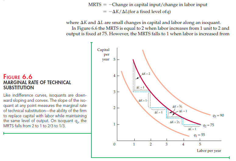
2 units to 3, and then declines to 2/3 and to 1/3.  Clearly, as more and more labor replaces capital, labor becomes less productive and capital becomes relatively more productive. Therefore, we need less capital to keep output constant, and the isoquant becomes flatter.

DIMINISHING  MRTS We assume that there is a diminishing MRTS. In other words, the MRTS falls as we move down along an isoquant. The mathemati- cal implication is that isoquants, like indifference curves, are convex, or bowed inward. This is indeed the case for most production technologies. The dimin- ishing MRTS tells us that the productivity of any one input is limited. As more and more labor is added to the production process in place of capital, the productivity of labor falls. Similarly, when more capital is added in place of labor, the productivity of capital falls. Production needs a balanced mix of both inputs.

As our discussion has just suggested, the MRTS is closely related to the mar­ginal products of labor MP_L and capital MP_K. To see how, imagine adding some labor and reducing the amount of capital sufficient to keep output constant. The additional output resulting from the increased labor input is equal to the addi­tional output per unit of additional labor (the marginal product of labor) times the number of units of additional labor:

Similarly, the decrease in output resulting from the reduction in capital is the loss of output per unit reduction in capital (the marginal product of capital) times the number of units of capital reduction:

Because we are keeping output constant by moving along an isoquant, the total change in output must be zero. Thus,

Equation (6.2) tells us that the marginal rate of technical substitution between two inputs is equal to the ratio of the marginal products of the inputs. This formula will be useful when we look at the firm’s cost-minimizing choice of inputs in Chapter 7.

5. Production Functions—Two  Special Cases

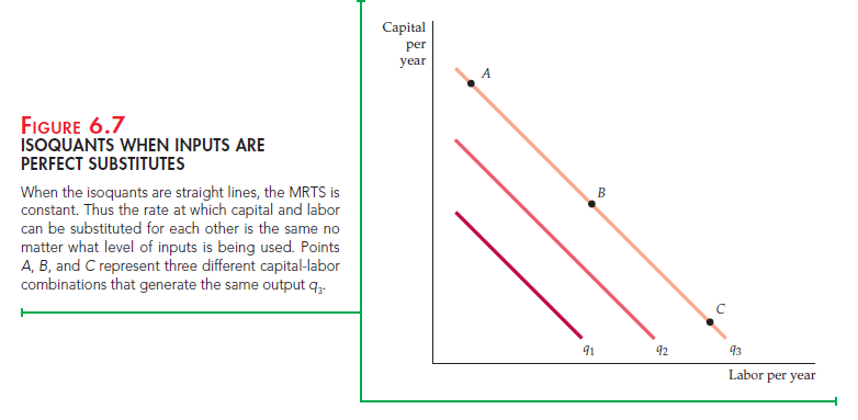
Two extreme cases of production functions show the possible range of input substitution in the production process. In the first case, shown in Figure 6.7, inputs to production are perfect substitutes for one another. Here the MRTS is constant at all points on an isoquant. As a result, the same output (say q3) can be produced with mostly capital (at A), with mostly labor (at C), or with a bal- anced combination of both (at B). For example, musical instruments can be man-

ufactured almost entirely with machine tools or with very few tools and highly skilled labor.

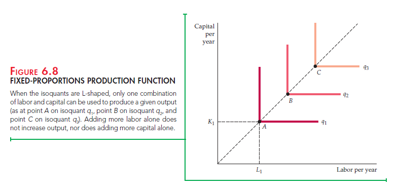
Figure 6.8 illustrates the opposite extreme, the fixed-proportions produc- tion function, sometimes called a Leontief production function. In this case,

ounce of nuts for every four ounces of oats in every serving. If the company were to purchase additional nuts but not additional oats, the output of cereal would remain unchanged, since the nuts must be combined with the oats in a fixed proportion. Similarly, purchasing additional oats without additional nuts would also be unproductive.

In Figure 6.8 points A, B, and C represent technically efficient combinations of inputs. For example, to produce output q1, a quantity of labor L1  and capital K1  can be used, as at A. If capital stays fixed at K1, adding more labor does not change output. Nor does adding capital with labor fixed at L1. Thus, on the ver- tical and the horizontal segments of the L-shaped isoquants, either the marginal product of capital or the marginal product of labor is zero. Higher output results only when both labor and capital are added, as in the move from input combi- nation A to input combination B.

The fixed-proportions production function describes situations in which methods of production are limited. For example, the production of a television show might involve a certain mix of capital (camera and sound equipment, etc.) and labor (producer, director, actors, etc.). To make more television shows, all inputs to production must be increased proportionally. In particular, it would be difficult to increase capital inputs at the expense of labor, because actors are necessary inputs to production (except perhaps for animated films). Likewise, it would be difficult to substitute labor for capital, because filmmaking today requires sophisticated film equipment.

Source: Pindyck Robert, Rubinfeld Daniel (2012), Microeconomics, Pearson, 8th edition.