Many firms are integrated—they consist of several divisions, each with its own managers. Some firms are horizontally integrated: There are several divisions that produce the same or closely related products. We saw an example of this when we discussed the multi-plant firm in Section 10.1. Some firms are verti- cally integrated: They have several divisions, with some divisions producing parts and components which other divisions use to produce the finished prod- uct. For example, automobile companies have “upstream” divisions that pro- duce engines, brakes, radiators and other components that the “downstream” divisions use to produce the finished cars. (Some firms are both vertically and horizontally integrated.)
This appendix explains the economic issues that arise in a vertically inte- grated firm. As we will see, vertical integration has important benefits, but it also introduces complex pricing decisions: How should the firm value the parts and components that are transferred from the upstream to the downstream divi- sions? The firm must determine transfer prices, the internal prices at which the parts and components from upstream divisions are “sold” to downstream divi- sions. Transfer prices must be chosen correctly because they are the signals that divisional managers use to determine output levels.
We will begin by explaining the advantages of vertical integration—advan- tages to the firm, as well as to the consumers who buy the end products of the firm. Some firms, however, are not vertically integrated; they simply buy parts and components from other independent firms. To understand why, we will explain some of the problems associated with vertical integration. Next, we will explain transfer pricing, and show how a vertically integrated firm should choose its transfer prices in a way that maximizes the firm’s total profit.
1. Why Vertically Integrate?
There are a number of advantages to vertical integration. If upstream and down- stream divisions are part of the same firm, it might be easier to guarantee that parts and components are produced and delivered on time, and are made to the precise specifications needed by the downstream division. (On the other hand, a carefully written and enforced contract between independent upstream and downstream firms can often achieve the same thing.) The biggest advantage of vertical integration, however, is that it avoids the problem of “double marginali- zation,” i.e., it avoids a double markup.
Market Power and Double Marginalization
Often, one or more firms selling to each other along a vertical chain will have mar- ket power. For example, United Technologies and General Electric have monop- oly power in the production of jet aircraft engines, which they sell to Boeing and Airbus, which in turn have monopoly power in the market for commercial aircraft. How do firms along a vertical chain exercise such monopoly power, and how are prices and output affected? Would the firms benefit from a vertical merger that integrates an upstream and a related downstream business? Would consumers?
To answer these questions, consider the following example. Suppose an engine manufacturer has monopoly power in the market for engines, and an automobile manufacturer that buys these engines has monopoly power in the market for its cars. Would this market power cause these two firms to benefit in any way if they were to merge? Would consumers of the final product—auto- mobiles—be better or worse off if the two companies merged? Many people (who haven’t read this book) would answer “maybe” to the first question, and “worse off” to the second question. It turns out, however, that when there is market power of this sort, a vertical merger can be beneficial to the two firms, and also beneficial to consumers.
SEPARATE FIRMS To see this, consider the following simple example. Suppose a monopolist producer of specialty engines produces those engines at a constant marginal cost cE, and sells the engines at a price PE. The engines are bought by a monopolist producer of sports cars, which sells the cars at the price P. Demand for the cars is given by
Q = A – P (A11.1)
with the constant A > cE. To keep this example as simple as possible, we will assume that the automobile manufacturer has no additional costs other than the cost of the engine. (As an exercise, you can repeat this example assuming that there is an additional constant marginal cost cA to assemble the cars.)
If the two companies are independent of each other, the automobile manufacturer will take the price of engines as given, and choose a price for its cars to maximize its profits:

You can check that given PE, the profit maximizing price of cars is:1

Then the number of cars sold and the automobile company’s profit are:

What about the engine manufacturer? It chooses the price of engines, PE, to maximize its profit:

You can confirm that the profit-maximizing price of engines is:

The profit to the engine manufacturer is then equal to:

Now go back to Equation (A11.5) for the profit to the automobile manufacturer, and substitute in Equation (A11.7) for the price of engines. You will see that the automobile company’s profit is then:

Hence the total profit for the two companies is:

Also, the price of cars paid by consumers is:

VERTICAL INTEGRATION Now suppose that the engine company and the automobile company merge to form a vertically integrated firm. The management of this firm would choose a price of automobiles to maximize the firm’s profit:
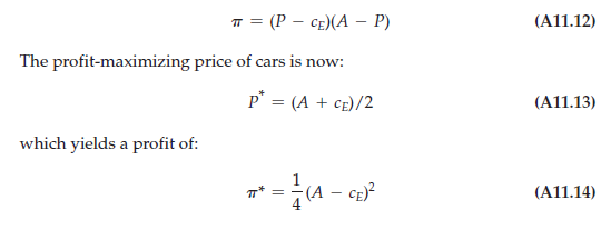
Observe that the profit for the integrated firm is greater than the total profit for the two individual firms that operate independently. Furthermore, the price to consumers for automobiles is lower. (To confirm that this is indeed the case, compare (A11.11) with (A11.13) and remember that A > cE.) Hence, in this case vertical integration benefits not only the merging firms, but also consumers. When each firm in a vertical chain marks up its price above its marginal cost, thereby increasing the price of the final product.
DOUBLE MARGINALIZATION Why would a vertical merger make both the merging firms and consumers better off? The reason is that vertical integration avoids the problem of double marginalization. When the two firms operate independently, each one exercises its monopoly power by marking up its price above its marginal cost. But to do this, each firm must contract its output. The engine producer contracts its output to mark up its price above its marginal cost, and then the automobile manufacturer does likewise. This “double marginaliza- tion” pushes the price above the “single marginalization” or single markup over price of the integrated firm.
This example of double marginalization is illustrated graphically in Figure A11.1, which shows the demand curve (average revenue curve) for cars, and the corresponding marginal revenue curve. For the automobile company, the marginal revenue curve for cars is the demand curve for engines (effec- tively, the net marginal revenue for engines). It describes the number of engines that the auto maker will buy as a function of price. From the point of view of the engine company, it is the average revenue curve for engines (i.e., the demand curve for engines that the engine company faces). Corresponding to that demand curve is the engine company’s marginal revenue curve for engines, labeled MRE in the figure. If the engine company and automobile company are separate entities, the engine company will produce a quantity of engines at the point where its marginal revenue curve intersects its marginal cost curve. That
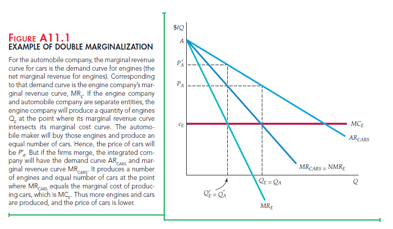
quantity of engines is labeled Q’E. The automobile maker will buy those engines and produce an equal number of cars. Hence, the price of cars will be PA’.
What happens if the two companies merge? The integrated company will have the demand curve ARCARS and the corresponding marginal revenue curve MRCARS. It will produce a number of engines and equal number of cars at the point where the marginal revenue curve for cars intersects the marginal cost of producing cars, which in this example is simply the marginal cost of engines. As shown in the figure, there will be a larger quantity of engines and cars produced at a correspondingly lower price.
ALTERNATIVES TO VERTICAL INTEGRATION What can firms do to reduce the problem of double marginalization if a vertical merger is not an option? One solution is for the upstream firm to try to make the downstream market as com- petitive as possible, thereby reducing any double marginalization. Thus, Intel, which has monopoly power in processors, would like to do everything it can to make sure that the market for personal computers remains highly competitive, and might even help computer firms that are in danger of going out of business.
A second method of dealing with double marginalization is called quantity forcing. The idea is to impose a sales quota or other restriction on downstream firms so that they cannot reduce their output in an attempt to marginalize. For example, automobile companies will create financial incentives to push dealer- ships (which have some monopoly power) to sell as many cars as possible.
2. Transfer Pricing in the Integrated Firm
We now turn to the profit-maximizing vertically integrated firm and see how it should choose its transfer prices and divisional output levels. We begin with the simplest case: There is no outside market for the output of the upstream divi- sion; i.e., the upstream division produces a good that is neither produced nor used by any other firm. Later we will consider what happens when there is an outside market for the upstream division’s output.
Transfer Pricing When There Is No Outside Market
Look again at Figure A11.1. We saw that if the firm is integrated, the profit- maximizing number of engines and cars it will produce is QE = QA, at the point where MRCARS equals the marginal cost of producing cars, which is MCE. Now suppose the downstream automobile division had to “pay” the upstream engine division a transfer price for each engine it used. What should that transfer price be? It should equal the marginal cost of producing engines, i.e., MCE. Why? Because then the automobile division will have a marginal cost of producing cars equal to MCE, so that even if it is left to maximize its own divisional profit, it will produce the correct number of cars.
Another way to see this is in terms of opportunity cost. What is the opportu- nity cost to the integrated firm of utilizing one more engine (to produce one more car)? It is the marginal cost of engines. Thus we have a simple rule: Set the transfer price of any upstream parts and components equal to the marginal cost of pro- ducing those parts and components.
You might argue that the example illustrated in Figure A11.1 is oversimpli- fied because the only cost of producing a car is the cost of an engine. So now consider a firm with three divisions: Two upstream divisions produce inputs to a downstream processing division. The two upstream divisions produce quantities Q1 and Q2 and have total costs C1(Q1) and C2(Q2). The downstream division produces a quantity Q using the production function
Q = f(K, L, Qi, Q2)
where K and L are capital and labor inputs, and Q1 and Q2 are the intermediate inputs from the upstream divisions. Excluding the costs of the inputs Q1 and Q2, the downstream division has a total production cost Cd(Q). Total revenue from sales of the final product is R(Q).
We assume there are no outside markets for the intermediate inputs Q2and Q2; they can be used only by the downstream division. Then the firm has two problems:
- What quantities Q2, Q2, and Q will maximize its profit?
- Is there an incentive scheme that will decentralize the firm’s management? In particular, is there a set of transfer prices P1 and P2, so that if each division maximizes its own divisional profit, the profit of the overall firm will also be maximized?
To solve these problems, we note that the firm’s total profit is
![]()
What is the level of Q1 that maximizes this profit? It is the level at which the cost of the last unit of Q1 is just equal to the additional revenue it brings to the firm. The cost of producing one extra unit of Q1 is the marginal cost A C1/ A Q1 = MCr How much extra revenue results from that one extra unit? An extra unit of Q1 allows the firm to produce more final output Q of an amount AQ/AQ1 = MP2, the marginal product of Qr An extra unit of final output results in additional revenue A R/A Q = MR, but it also results in additional cost to the downstream division of an amount AC/ AQ = MCd. Thus the net marginal revenue NMR1 that the firm earns from an extra unit of Q1 is (MR – MCd)MPr Setting this equal to the marginal cost of the unit, we obtain the following rule for profit maximization4:
NMR1 = (MR – MCd)MP1 = MC1 (A11.16)
Going through the same steps for the second intermediate input gives
NMR2 = (MR – MCd)MP2 = MC2 (A11.17)
Note from equations (A11.16) and (A11.17) that it is incorrect to determine the firm’s final output level Q by setting marginal revenue equal to marginal cost for the downstream division—i.e., by setting MR = MCd. Doing so ignores the cost of producing the intermediate input. (MR exceeds MCd because this cost is positive.) Also, note that equations (A11.16) and (A11.17) are standard conditions of marginal analysis: The output of each upstream division should be such that its marginal cost is equal to its marginal contribution to the profit of the overall firm.
Now, what transfer prices P1 and P2 should be “charged” to the downstream division for its use of the intermediate inputs? Remember that if each of the three divisions uses these transfer prices to maximize its own divisional profit, the profit of the overall firm should be maximized. The two upstream divisions will maximize their divisional profits, p and p2, which are given by

Because the upstream divisions take Pi and P2 as given, they will choose Qi and Q2 so that Pi = MCi and P2 = MC2. Similarly, the downstream division will maximize
![]()
Because the downstream division also takes Pi and P2 as given, it will choose Qi and Q2 so that

Note that by setting the transfer prices equal to the respective marginal costs (Pj = MCj and P2 = MC2), the profit-maximizing conditions given by equations (Aii.i6) and (Aii.i7) will be satisfied. We therefore have a simple solution to the transfer pricing problem: Set each transfer price equal to the marginal cost of the respective upstream division. Then when each division is required to maximize its own profit, the quantities Qi and Q2 that the upstream divisions will want to produce will be the same quantities that the downstream division will want to “buy,” and they will maximize the firm’s total profit.
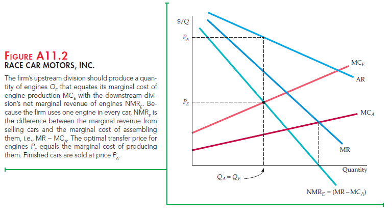
To illustrate this graphically, suppose Race Car Motors, Inc., has two divisions. The upstream Engine Division produces engines, and the downstream Assembly Division puts together automobiles, using one engine (and a few other parts) in each car. In Figure Aii.2, the average revenue curve AR is Race Car Motors’ demand curve for cars. (Note that the firm has monopoly power in the automobile market.) MCA is the marginal cost of assembling automobiles, given the engines (i.e., it does not include the cost of the engines). Because the car requires one engine, the marginal product of the engines is one. Thus the curve labeled MR – MCA is also the net marginal revenue curve for engines:
![]()
The profit-maximizing number of engines (and number of cars) is given by the intersection of the net marginal revenue curve NMRE with the marginal cost curve for engines MCr Having determined the number of cars that it will produce, and knowing its divisional cost functions, the management of Race Car Motors can now set the transfer price PE that correctly values the engines used to produce its cars. This is the transfer price that should be used to calculate divisional profit (and year-end bonuses for divisional managers).
Transfer Pricing with a Competitive Outside Market
Now suppose there is a competitive outside market for the intermediate good produced by an upstream division. Because the outside market is competitive, there is a single market price at which one can buy or sell the good. Therefore, the marginal cost of the intermediate good is simply the market price. Because the optimal transfer price must equal marginal cost, it must also equal the competitive market price.
To see this, suppose there is a competitive market for the engines that Race Car Motors produces. If the market price is low, Race Car Motors may want to buy some or all of its engines in the market; if it is high, it may want to sell engines in the market. Figure A11.3 illustrates the first case. For quantities below Qe 1, the upstream division’s marginal cost of producing engines MCE is below the market price PE,M; for quantities above QE,1, it is above the market price. The firm should obtain engines at the least cost, so the marginal cost of engines MCE will be the upstream division’s marginal cost for quantities up to QE,1 and the market price for quantities above QE,1. Note that Race Car Motors uses more engines and produces more cars than it would have had there been no outside engine market. The downstream division now buys QE 2 engines and produces an equal number of automobiles. However, it “buys” only QE1 of these engines from the upstream division and the rest on the open market.
It might seem strange that Race Car Motors must go into the open market to buy engines that it can make itself. If it made all of its own engines, however, its marginal cost of producing them would exceed the competitive market price. Although the profit of the upstream division would be higher, the total profit of the firm would be lower.
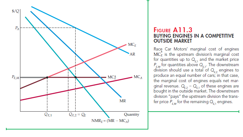
Figure A11.4 shows the case where Race Car Motors sells engines in the outside market. Now the competitive market price PE M is above the transfer price that the firm would have set had there been no outside market. In this case, although the upstream Engine Division produces QE 2 engines, only QE 2 engines are used by the downstream division to produce automobiles. The rest are sold in the outside market at the price PE,M.
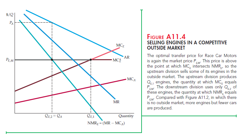
Note that compared with a situation in which there is no outside engine mar-ket, Race Car Motors is producing more engines but fewer cars. Why not pro-duce this larger number of engines but use all of them to produce more cars?
Because the engines are too valuable. On the margin, the net revenue that can be earned from selling them in the outside market is higher than the net revenue from using them to build additional cars.
Transfer Pricing with a Noncompetitive
Outside Market
Now suppose there is an outside market for the output of the upstream divi- sion, but that market is not competitive. Suppose that the engines produced by the upstream Engine Division is a special one that only Race Car Motors can make, so that Race Car Motors can be a monopoly supplier to that outside market while also producing engines for its own use. We will not work through the details of this case, but you should be able to see that the transfer price paid to the Engine Division will be below the price at which engines are bought in the outside market. Why “pay” the Engine Division a price that is lower than that paid in the outside market? The reason is that the opportunity cost of uti- lizing an engine internally is just the marginal cost of producing the engine, whereas the opportunity cost of selling it outside is higher, because it includes a monopoly markup.
Sometimes a vertically integrated firm can buy components in an outside market in which it has monopsony power. Suppose, for example, that Race Car Motors is the only company that uses the engines produced by its upstream Engine Division, but other companies also make that engine. Thus Race Car Motors can obtain its engines from its upstream Engine Division, or can pur- chase them as a monopsonist in the outside market. You should be able to see that in this case, the transfer price paid to the Engine Division will be above the price at which engines are bought in the outside market. Why “pay” the upstream division a price that is higher than that paid in the outside market? With mon- opsony power, purchasing one additional engine in the outside market incurs a marginal expenditure that is greater than the actual price paid in that market. (The marginal expenditure is higher because purchasing an additional unit raises the average expenditure paid for all units bought in the outside market.) The marginal expenditure is the opportunity cost of buying an engine outside, and therefore should equal the transfer price paid to the Engine Division, so the transfer price will be greater than the price paid outside.
Taxes and Transfer Pricing
So far we have ignored taxes in our discussion of transfer pricing. But in fact taxes can play an important role in determining transfer prices when the objective is to maximize the after-tax profits of the integrated firm. This is especially the case when the upstream and downstream divisions of the firm operate in different countries.
To see this, suppose that the upstream Engine Division of Race Car Motors happens to be located in an Asian country with a low corporate profits tax rate, while the downstream Assembly Division is located in the United States, with a higher tax rate. Suppose that in the absence of taxes, the marginal cost and thus the optimal transfer price for an engine is $5000. How would this transfer price be affected by taxes?
In our example, the difference in tax rates will cause the opportunity cost of using an engine downstream to exceed $5000. Why? Because the downstream profit generated by the use of the engine will be taxed at a relatively high rate. Thus, taking taxes into account, the firm will want to set a higher transfer price, perhaps $7000. This will reduce the downstream profits in the United States (so that the firm will pay less in taxes) and increase the profits of the upstream divi- sion, which faces a lower tax rate.
3. A Numerical Example
Suppose Race Car Motors has the following demand for its automobiles:
P = 20,000 – Q
Its marginal revenue is thus
MR = 20,000 – 2Q
The downstream division’s cost of assembling cars is
Ca(Q) = 8000Q
so that the division’s marginal cost is MCA = 8000. The upstream division’s cost of producing engines is
Ce(Qe) = 2Q2e
The division’s marginal cost is thus MCE(QE) = 4QE.
First, suppose there is no outside market for the engines. How many engines and cars should the firm produce? What should be the transfer price for engines? To solve this problem, we set the net marginal revenue for engines equal to the marginal cost of producing engines. Because each car has one engine, QE = Q. The net marginal revenue of engines is thus
NMRe = MR – MCa = 12,000 – 2QE
Now set NMRe equal to MCE:
12,000 – 2Qe = 4Qe
Thus 6Qe = 12,000 and QE = 2000. The firm should therefore produce 2000 engines and 2000 cars. The optimal transfer price is the marginal cost of these 2000 engines:
Pe = 4Qe = $8000
Second, suppose that engines can be bought or sold for $6000 in an outside competitive market. This is below the $8000 transfer price that is optimal when there is no outside market, so the firm should buy some engines outside. Its marginal cost of engines, and the optimal transfer price, is now $6000. Set this $6000 marginal cost equal to the net marginal revenue of engines:
6000 = NMRe = 12,000 – 2Qe
Thus the total quantity of engines and cars is now 3000. The company now produces more cars (and sells them at a lower price) because its cost of engines is lower. Also, since the transfer price for the engines is now $6000, the upstream Engine Division supplies only 1500 engines (because MCE(1500) = $6000). The remaining 1500 engines are bought in the outside market.
Source: Pindyck Robert, Rubinfeld Daniel (2012), Microeconomics, Pearson, 8th edition.

certainly like your web-site but you have to test the spelling on several of your posts. Several of them are rife with spelling problems and I to find it very bothersome to inform the reality nevertheless I will definitely come back again.