Price Competition

We have assumed that our oligopolistic firms compete by setting quantities. In many oligopolistic industries, however, competition occurs along price dimen- sions. For example, automobile companies view price as a key strategic variable, and each one chooses its price with its competitors in mind. In this section, we use the Nash equilibrium concept to study price competition, first in an industry that produces a homogeneous good and then in an industry with some degree of product differentiation.

1. Price Competition with Homogeneous

Products—The Bertrand Model

The Bertrand model was developed in 1883 by another French economist, Joseph Bertrand. Like the Cournot model, it applies to firms that produce the same homogeneous good and make their decisions at the same time. In this case, however, the firms choose prices instead of quantities. As we will see, this change can dramatically affect the market outcome.

Let’s return to the duopoly example of the last section, in which the market demand curve is

P = 30 – Q

where Q = Q1  + Q2  is again total production of a homogeneous good. This time, however, we will assume that both firms have a marginal cost of $3:

MC 1  = MC 2  =  $3

As an exercise, you can show that the Cournot equilibrium for this duopoly, which results when both firms choose output simultaneously, is Q1 = Q2 = 9. You can also check that in this Cournot equilibrium, the market price is $12, so that each firm makes a profit of $81.

Now suppose that these two duopolists compete by simultaneously choosing a price instead of a quantity. What price will each firm choose, and how much profit will each earn? To answer these questions, note that because the good is homogeneous, consumers will purchase only from the lowest-price seller. Thus, if the two firms charge different prices, the lower-price firm will supply the entire market and the higher-price firm will sell nothing. If both firms charge the same price, consumers will be indifferent as to which firm they buy from and each firm will supply half the market.

What is the Nash equilibrium in this case? If you think about this problem a little, you will see that because of the incentive to cut prices, the Nash equilibrium is the competitive outcome—i.e., both firms set price equal to marginal cost: P1 = P2 = $3. Then industry output is 27 units, of which each firm produces 13.5 units. And because price equals marginal cost, both firms earn zero profit. To check that this outcome is a Nash equilibrium, ask whether either firm would have any incentive to

change its price. Suppose Firm 1 raised its price. It would then lose all of its sales to Firm 2 and therefore be no better off. If, instead, it lowered its price, it would capture the entire market but would lose money on every unit it produced; again, it would be worse off. Therefore, Firm 1 (and likewise Firm 2) has no incentive to deviate: It is doing the best it can to maximize profit, given what its competitor is doing.

Why couldn’t there be a Nash equilibrium in which the firms charged the same price, but a higher one (say, $5), so that each made some profit? Because if either firm lowered its price just a little, it could capture the entire market and nearly double its profit. Thus each firm would want to undercut its competitor. Such undercutting would continue until the price dropped to $3.

By changing the strategic choice variable from output to price, we get a dramatically different outcome. In the Cournot model, because each firm pro- duces only 9 units, the market price is $12. Now the market price is $3. In the Cournot model, each firm made a profit; in the Bertrand model, the firms price at marginal cost and make no profit.

The Bertrand model has been criticized on several counts. First, when firms produce a homogeneous good, it is more natural to compete by setting quantities rather than prices. Second, even if firms do set prices and choose the same price (as the model predicts), what share of total sales will go to each one? We assumed that sales would be divided equally among the firms, but there is no reason why this must be the case. Despite these shortcomings, the Bertrand model is useful because it shows how the equilibrium outcome in an oligopoly can depend cru- cially on the firms’ choice of strategic variable.2

2. Price Competition with Differentiated Products

Oligopolistic markets often have at least some degree of product differentia- tion.3 Market shares are determined not just by prices, but also by differences in the design, performance, and durability of each firm’s product. In such cases, it is natural for firms to compete by choosing prices rather than quantities.

To see how price competition with differentiated products can work, let’s go through the following simple example. Suppose each of two duopolists has fixed costs of $20 but zero variable costs, and that they face the same demand curves:

Firm 1=s demand:   Q1  = 12 – 2P1  + P2                                         (12.5a)

Firm 2=s demand:   Q2  = 12 – 2P2  + P1                                        (12.5b)

where P1  and P2  are the prices that Firms 1 and 2 charge, respectively, and Q1 and Q2 are the resulting quantities that they sell. Note that the quantity that each firm can sell decreases when it raises its own price but increases when its com- petitor charges a higher price.

CHOOSING PRICES We will assume that both firms set their prices at the same time and that each firm takes its competitor ’s price as fixed. We can therefore use the Nash equilibrium concept to determine the resulting prices. Let’s begin with Firm 1. Its profit p1 is its revenue P1Q1 less its fixed cost of $20. Substituting for Q1 from the demand curve of equation (12.5a), we have

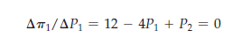
At what price P1 is this profit maximized? The answer depends on P2, which Firm 1 assumes to be fixed. However, whatever price Firm 2 is charging, Firm 1’s profit is maximized when the incremental profit from a very small increase in its own price is just zero. Taking P2 as fixed, Firm 1’s profit-maximizing price is therefore given by

This equation can be rewritten to give the following pricing rule, or reaction curve, for Firm 1:

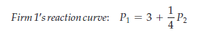
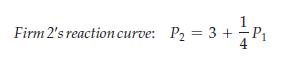
This equation tells Firm 1 what price to set, given the price P2  that Firm 2 is set- ting. We can similarly find the following pricing rule for Firm 2:

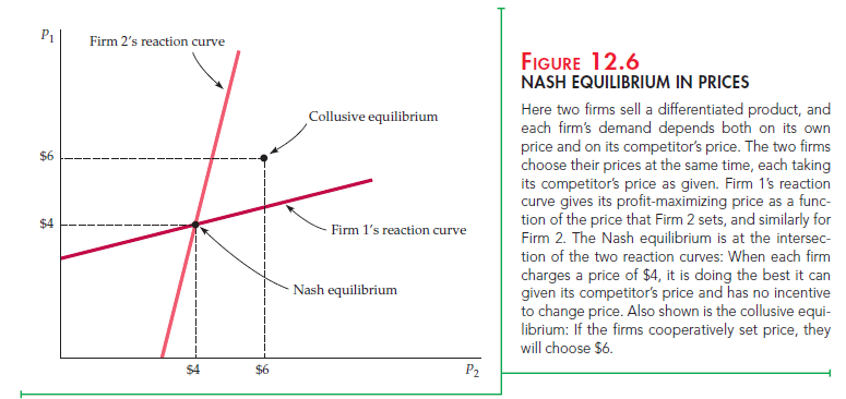
These reaction curves are drawn in Figure 12.6. The Nash equilibrium is at the point where the two reaction curves cross; you can verify that each firm is then charging a price of $4 and earning a profit of $12. At this point, because each firm is doing the best it can given the price its competitor has set, neither firm has an incentive to change its price.

Now suppose the two firms collude: Instead of choosing their prices inde- pendently, they both decide to charge the same price—namely, the price that maximizes both of their profits. You can verify that the firms would then charge $6, and that they would be better off colluding because each would now earn a profit of $16.4 Figure 12.6 shows this collusive equilibrium.

Finally, suppose Firm 1 sets its price first and that, after observing Firm 1’s deci- sion, Firm 2 makes its pricing decision. Unlike the Stackelberg model in which the firms set their quantities, in this case Firm 1 would be at a distinct disadvantage by moving first. (To see this, calculate Firm 1’s profit-maximizing price, taking Firm 2’s reaction curve into account.) Why is moving first now a disadvantage? Because it gives the firm that moves second an opportunity to undercut slightly and thereby capture a larger market share. (See Exercise 11 at the end of the chapter.)

Source: Pindyck Robert, Rubinfeld Daniel (2012), Microeconomics, Pearson, 8th edition.