Oligopoly

In oligopolistic markets, the products may or may not be differentiated. What matters is that only a few firms account for most or all of total production. In some oligopolistic markets, some or all firms earn substantial profits over the long run because barriers to entry make it difficult or impossible for new firms to enter. Oligopoly is a prevalent form of market structure. Examples of oligopolistic industries include automobiles, steel, aluminum, petrochemicals, electrical equipment, and computers.

Why might barriers to entry arise? We discussed some of the reasons in Chapter 10. Scale economies may make it unprofitable for more than a few firms to coexist in the market; patents or access to a technology may exclude potential competitors; and the need to spend money for name recognition and market reputation may discourage entry by new firms. These are “natural” entry barriers—they are basic to the structure of the particular market. In addi- tion, incumbent firms may take strategic actions to deter entry. For example, they might threaten to flood the market and drive prices down if entry occurs, and to make the threat credible, they can construct excess production capacity.

Managing an oligopolistic firm is complicated because pricing, output, adver- tising, and investment decisions involve important strategic considerations. Because only a few firms are competing, each firm must carefully consider how its actions will affect its rivals, and how its rivals are likely to react.

Suppose that because of sluggish car sales, Ford is considering a 10-percent price cut to stimulate demand. It must think carefully about how competing auto companies will react. They might not react at all, or they might cut their prices only slightly, in which case Ford could enjoy a substantial increase in sales, largely at the expense of its competitors. Or they might match Ford’s price cut, in which case all of the firms will sell more cars, but might make much lower profits because of the lower prices. Another possibility is that some firms will cut their prices by even more than Ford to punish Ford for rocking the boat, and this in turn might lead to a price war and to a drastic fall in profits for the entire industry. Ford must carefully weigh all these possibilities. In fact, for almost any major economic decision that a firm makes—setting price, determin- ing production levels, undertaking a major promotion campaign, or investing in new production capacity—it must try to determine the most likely response of its competitors.

These strategic considerations can be complex. When making decisions, each firm must weigh its competitors’ reactions, knowing that these competitors will also weigh its reactions to their decisions. Furthermore, decisions, reactions, reactions to reactions, and so forth are dynamic, evolving over time. When the managers of a firm evaluate the potential consequences of their decisions, they must assume that their competitors are as rational and intelligent as they are. Then, they must put themselves in their competitors’ place and consider how they would react.

1. Equilibrium in an Oligopolistic Market

When we study a market, we usually want to determine the price and quantity that will prevail in equilibrium. For example, we saw that in a perfectly com- petitive market, the equilibrium price equates the quantity supplied with the quantity demanded. Then we saw that for a monopoly, an equilibrium occurs when marginal revenue equals marginal cost. Finally, when we studied monop- olistic competition, we saw how a long-run equilibrium results as the entry of new firms drives profits to zero.

In these markets, each firm could take price or market demand as given and largely ignore its competitors. In an oligopolistic market, however, a firm sets price or output based partly on strategic considerations regarding the behavior of its competitors. At the same time, competitors’ decisions depend on the first firm’s decision. How, then, can we figure out what the market price and output will be in equilibrium—or whether there will even be an equilibrium? To answer these questions, we need an underlying principle to describe an equilibrium when firms make decisions that explicitly take each other ’s behavior into account.

Remember how we described an equilibrium in competitive and monopo- listic markets: When a market is in equilibrium, firms are doing the best they can and have no reason to change their price or output. Thus a competitive market is in equi- librium when the quantity supplied equals the quantity demanded: Each firm is doing the best it can—it is selling all that it produces and is maximizing its profit. Likewise, a monopolist is in equilibrium when marginal revenue equals marginal cost because it, too, is doing the best it can and is maximizing its profit.

NASH EQUILIBRIUM With some modification, we can apply this same princi- ple to an oligopolistic market. Now, however, each firm will want to do the best it can given what its competitors are doing. And what should the firm assume that its competitors are doing? Because the firm will do the best it can given what its competitors are doing, it is natural to assume that these competitors will do the best they can given what that firm is doing. Each firm, then, takes its competitors into account, and assumes that its competitors are doing likewise.

This may seem a bit abstract at first, but it is logical, and as we will see, it gives us a basis for determining an equilibrium in an oligopolistic market. The concept was first explained clearly by the mathematician John Nash in 1951, so we call the equilibrium it describes a Nash equilibrium. It is an important con- cept that we will use repeatedly:

Nash Equilibrium: Each firm is doing the best it can given what its competitors are doing.

We discuss this equilibrium concept in more detail in Chapter 13, where we show how it can be applied to a broad range of strategic problems. In this chap- ter, we will apply it to the analysis of oligopolistic markets.

To keep things as uncomplicated as possible, this chapter will focus largely on markets in which two firms are competing with each other. We call such a market a duopoly. Thus each firm has just one competitor to take into account in making its decisions. Although we focus on duopolies, our basic results will also apply to markets with more than two firms.

2. The Cournot Model

We will begin with a simple model of duopoly first introduced by the French economist Augustin Cournot in 1838. Suppose the firms produce a homoge- neous good and know the market demand curve. Each firm must decide how much to produce, and the two firms make their decisions at the same time. When making its production decision, each firm takes its competitor into account. It knows that its competitor is also deciding how much to produce, and the market price will depend on the total output of both firms.

The essence of the Cournot model is that each firm treats the output level of its competitor as fixed when deciding how much to produce. To see how this works, let’s consider the output decision of Firm 1. Suppose Firm 1 thinks that Firm 2 will produce nothing. In that case, Firm 1’s demand curve is the market demand curve. In Figure 12.3 this is shown as D₁(0), which means the demand curve for Firm 1, assuming Firm 2 produces zero. Figure 12.3 also shows the correspond­ing marginal revenue curve MR₁(0). We have assumed that Firm 1’s marginal cost MCj is constant. As shown in the figure, Firm 1’s profit-maximizing output is 50 units, the point where MR₁(0) intersects MC₁. So if Firm 2 produces zero, Firm 1 should produce 50.

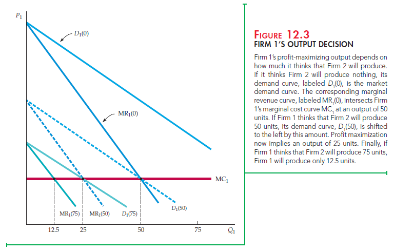
Suppose, instead, that Firm 1 thinks Firm 2 will produce 50 units. Then Firm 1’s demand curve is the market demand curve shifted to the left by 50. In Figure 12.3, this curve is labeled D₁(50), and the corresponding marginal reve­nue curve is labeled MR₁(50). Firm 1’s profit-maximizing output is now 25 units, the point where MR₁(50) = MC₁. Now, suppose Firm 1 thinks that Firm 2 will produce 75 units. Then Firm 1’s demand curve is the market demand curve shifted to the left by 75. It is labeled D₁(75) in Figure 12.3, and the corresponding marginal revenue curve is labeled MR₁(75). Firm 1’s profit-maximizing output is now 12.5 units, the point where MR₁(75) = MC₁. Finally, suppose Firm 1 thinks that Firm 2 will produce 100 units. Then Firm 1’s demand and marginal revenue curves (which are not shown in the figure) would intersect its marginal cost curve on the vertical axis; if Firm 1 thinks that Firm 2 will produce 100 units or more, it should produce nothing.

REACTION CURVES To summarize: If Firm 1 thinks that Firm 2 will produce nothing, it will produce 50; if it thinks Firm 2 will produce 50, it will produce 25; if it thinks Firm 2 will produce 75, it will produce 12.5; and if it thinks Firm 2 will produce 100, then it will produce nothing. Firm 1’s profit-maximizing output is thus a decreasing schedule of how much it thinks Firm 2 will produce. We call this schedule Firm 1’s reaction curve and denote it by Q*(Q₂). This curve is plotted in Figure 12.4, where each of the four output combinations that we found above is shown as an x.

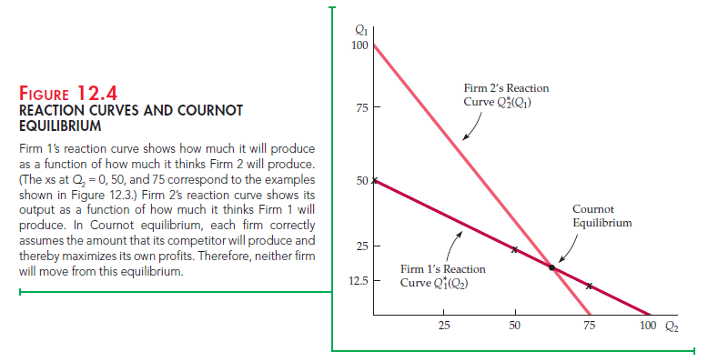
We can go through the same kind of analysis for Firm 2; that is, we can deter­mine Firm 2’s profit-maximizing quantity given various assumptions about how much Firm 1 will produce. The result will be a reaction curve for Firm 2—i.e., a schedule Q2(Qi) that relates its output to the output that it thinks Firm 1 will produce. If Firm 2’s marginal revenue or marginal cost curve is different from that of Firm 1, its reaction curve will also differ in form. For example, Firm 2’s reaction curve might look like the one drawn in Figure 12.4.

COURNOT EQUILIBRIUM How much will each firm produce? Each firm’s reaction curve tells it how much to produce, given the output of its competitor. In equilibrium, each firm sets output according to its own reaction curve; the equilibrium output levels are therefore found at the intersection of the two reac­tion curves. We call the resulting set of output levels a Cournot equilibrium. In this equilibrium, each firm correctly assumes how much its competitor will produce, and it maximizes its profit accordingly.

Note that this Cournot equilibrium is an example of a Nash equilibrium (and thus it is sometimes called a Cournot-Nash equilibrium). Remember that in a Nash equilibrium, each firm is doing the best it can given what its competitors are doing. As a result, no firm would individually want to change its behavior. In the Cournot equilibrium, each firm is producing an amount that maximizes its profit given what its competitor is producing, so neither would want to change its output.

Suppose the two firms are initially producing output levels that differ from the Cournot equilibrium. Will they adjust their outputs until the Cournot equi­librium is reached? Unfortunately, the Cournot model says nothing about the dynamics of the adjustment process. In fact, during any adjustment process, the model’s central assumption that each firm can assume that its competitor’s output is fixed will not hold. Because both firms would be adjusting their out­puts, neither output would be fixed. We need different models to understand dynamic adjustment, and we will examine some in Chapter 13.

When is it rational for each firm to assume that its competitor’s output is fixed? It is rational if the two firms are choosing their outputs only once because then their outputs cannot change. It is also rational once they are in Cournot equilibrium because then neither firm will have any incentive to change its out- put. When using the Cournot model, we must therefore confine ourselves to the behavior of firms in equilibrium.

3. The Linear Demand Curve—An Example

Let’s work through an example—two identical firms facing a linear market demand curve. This will help clarify the meaning of a Cournot equilibrium and let us compare it with the competitive equilibrium and the equilibrium that results if the firms collude and choose their output levels cooperatively.

Suppose our duopolists face the following market demand curve:

P = 30 – Q

where Q is the total production of both firms (i.e., Q = Q1  + Q2). Also, suppose that both firms have zero marginal cost:

MC 1  = MC 2  = 0

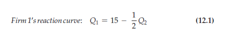
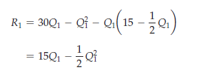
We can determine the reaction curve for Firm 1 as follows. To maximize profit, it sets marginal revenue equal to marginal cost. Its total revenue R1 is given by

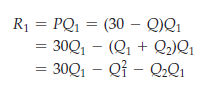
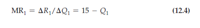
Its marginal revenue MR₁ is just the incremental revenue AR₁ resulting from an incremental change in output AQ₁:

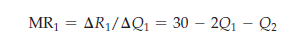
Now, setting MR1  equal to zero (the firm’s marginal cost) and solving for Q1, we find

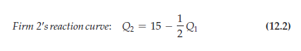
The same calculation applies to Firm 2:

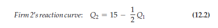
The equilibrium output levels are the values for Q1  and Q2  at the intersection of the two reaction curves—i.e., the levels that solve equations (12.1) and (12.2). By replacing Q2  in equation (12.1) with the expression on the righthand side of (12.2), you can verify that the equilibrium output levels are

Cournot equilibrium:   Q1  = Q2  = 10

The total quantity produced is therefore Q = Q₁ + Q₂ = 20, so the equilibrium market price is P = 30 – Q = 10, and each firm earns a profit of 100.

Figure 12.5 shows the firms’ reaction curves and this Cournot equilibrium. Note that Firm 1’s reaction curve shows its output Q₁ in terms of Firm 2’s output Q₂. Likewise, Firm 2’s reaction curve shows Q₂ in terms of Q₁. (Because the firms are identical, the two reaction curves have the same form. They look different because one gives Q₁ in terms of Q₂ and the other gives Q₂ in terms of Q₁.) The Cournot equilibrium is at the intersection of the two curves. At this point, each firm is maximizing its own profit, given its competitor’s output.

We have assumed that the two firms compete with each other. Suppose, instead, that the antitrust laws were relaxed and the two firms could collude. They would set their outputs to maximize total profit, and presumably they would split that profit evenly. Total profit is maximized by choosing total output Q so that marginal revenue equals marginal cost, which in this example is zero. Total revenue for the two firms is

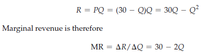
Setting MR equal to zero, we see that total profit is maximized when Q = 15.

Any combination of outputs Q1  and Q2  that add up to 15 maximizes total profit. The curve Q1  + Q2  = 15, called the collusion curve, therefore gives all pairs of outputs Q1  and Q2  that maximize total profit. This curve is also shown in

Figure 12.5. If the firms agree to share profits equally, each will produce half of the total output:

Q1  = Q2  = 7.5

As you would expect, both firms now produce less—and earn higher prof- its (112.50)—than in the Cournot equilibrium. Figure 12.5 shows this collusive equilibrium and the competitive output levels found by setting price equal to marginal cost. (You can verify that they are Q1 = Q2 = 15, which implies that each firm makes zero profit.) Note that the Cournot outcome is much better (for the firms) than perfect competition, but not as good as the outcome from collusion.

4. First Mover Advantage—The Stackelberg Model

We have assumed that our two duopolists make their output decisions at the same time. Now let’s see what happens if one of the firms can set its output first. There are two questions of interest. First, is it advantageous to go first? Second, how much will each firm produce?

Continuing with our example, we assume that both firms have zero marginal cost, and that market demand is given by P = 30 − Q, where Q is total output. Suppose Firm 1 sets its output first and then Firm 2, after observing Firm 1’s output, makes its output decision. In setting output, Firm 1 must therefore consider how Firm 2 will react. This Stackelberg model of duopoly is different from the Cournot model, in which neither firm has any opportunity to react.

Let’s begin with Firm 2. Because it makes its output decision after Firm 1, it takes Firm 1’s output as fixed. Therefore, Firm 2’s profit-maximizing output is given by its Cournot reaction curve, which we derived above as equation (12.2):

What about Firm 1? To maximize profit, it chooses Q1 so that its marginal rev- enue equals its marginal cost of zero. Recall that Firm 1’s revenue is

Because R1  depends on Q2, Firm 1 must anticipate how much Firm 2 will pro- duce. Firm 1 knows, however, that Firm 2 will choose Q2  according to the reac- tion curve (12.2). Substituting equation (12.2) for Q2 into equation (12.3), we find that Firm 1’s revenue is

R1 = PQ1 = 30Q1 – Q1 2 – Q2Q1                (12.3)

Its marginal revenue is therefore

Setting MR₁ = 0 gives Q₁ = 15. And from Firm 2’s reaction curve (12.2), we find that Q₂ = 7.5. Firm 1 produces twice as much as Firm 2 and makes twice as much profit. Going first gives Firm 1 an advantage. This may appear counterin­tuitive: It seems disadvantageous to announce your output first. Why, then, is going first a strategic advantage?

The reason is that announcing first creates a fait accompli: No matter what your competitor does, your output will be large. To maximize profit, your com­petitor must take your large output level as given and set a low level of output for itself. If your competitor produced a large level of output, it would drive price down and you would both lose money. So unless your competitor views “getting even” as more important than making money, it would be irrational for it to produce a large amount. As we will see in Chapter 13, this kind of “first­mover advantage” occurs in many strategic situations.

The Cournot and Stackelberg models are alternative representations of oligopolistic behavior. Which model is the more appropriate depends on the industry. For an industry composed of roughly similar firms, none of which has a strong operating advantage or leadership position, the Cournot model is prob- ably the more appropriate. On the other hand, some industries are dominated by a large firm that usually takes the lead in introducing new products or setting price; the mainframe computer market is an example, with IBM the leader. Then the Stackelberg model may be more realistic.

Source: Pindyck Robert, Rubinfeld Daniel (2012), Microeconomics, Pearson, 8th edition.