Poststratification Weights of Survey Data in Stata

The previous section gave an example of weights based on the sampling design, which was known before data collection began. A second type of weights might be defined after we have collected the data, and see that despite our best efforts, it appears unrepresentative in some respect. For instance, the sample might have a gender or age distribution noticeably different from those of our target population, making other results suspect. Poststratification refers to probability weights calculated so that the proportions of particular groups or strata in our sample more closely resemble the population.

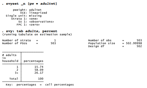
The Granite State Poll sample is 54.65% female. But according to the 2010 Census, the adult population of New Hampshire is only 51.6% female. If we guessed from the survey that the state’s population was something close to 54.65% female, we would be off the mark. Moreover, we could easily draw mistaken conclusions about other things correlated with gender, such as voting. This apparent response bias could undermine our ability to draw inferences about a larger population.

There are many ways to approach poststratification. (For an alternative to the by-hand approach shown below, Stata’s svyset command offers a poststrata option, illustrated in the Survey Reference Manual; type help svyset for the basic syntax.) If we know the true population percentages of key variables, as we do regarding gender, then weights to adjust for response bias can be calculated from population percentage divided by sample percentage. Sex is coded 0 for males, who make up 48.4% of the adult population of New Hampshire but only 45.35% of this sample. It is coded 1 for females, who are 51.6% of the population and 54.65% of the sample. There are no missing values of sex in these data.

We calculate weights slightly above one for males: 48.4/45.35 = 1.067. For females the weights are slightly below one: 51.6/54.65 = .944.

If we svyset the data using sexwt as the probability weight, svy: tab produces a weighted table showing exactly the right proportions of men (48.4%) and women (51.6%). After calculating poststratification weights, it is good to check on whether they perform as intended.

More elaborate poststratification weights could follow a similar approach. For example, suppose that for a different study we wish to approximate a population age-race-sex distribution.

1. Obtain a table of age-race-sex percentages from Census or other data on the population of interest, such as adults living in a particular state. If we employ five groups for age (18-29, 30-39, etc.) and two for race (white, nonwhite), this results in 20 numbers such as the percentage of that state’s adult population consisting of white males 18-29, the percentage of white females 18-29, and so forth.
2. Obtain a similar table of age-race-sex percentages from the sample, for example by creating and tabulating a new variable named ARS denoting age-race-sex combinations:

. egen ARS = group(agegroup race sex), lname(ars)

. tab ARS

3. Define a new set of weights, using generate … if commands. For example, suppose we know that 8.6% of the adult population in the study area consists of white males age 18-29, and 8.2% are white females in this age group. In our unweighted sample, however, we see only 2.6% white males 18-29, and 5.1% white females — so the young adults, particularly young males, are under-represented. We could create a new age-race-sex weight variable named ARSwt equal to 1 (a neutral weight) if we do not know a respondent’s age-race-sex combination, and otherwise equal to the population percentage divided by corresponding sample percentage for their age-race-sex group. The first few commands could be

. generate ARSwt = 1 if ARS >= .

. label variable ARSwt “Age-race-sex weights”

. replace ARSwt = 8.6/2.6 if ARS == 1 . replace ARSwt = 8.2/5.1 if ARS == 2

Poststratification adjustments work best in connection with carefully-designed surveys, and should not be misunderstood as a cure for haphazard sampling. Such adjustments have been applied most extensively in areas such as voter opinion polls and social science surveys, where great effort goes into securing the most representative samples to begin with. These also are areas where independent evidence such as vote outcomes or replications by other researchers provides reality tests for how well the adjustments succeed.

A single dataset might include weight variables calculated from more than one source, such as design weights and poststratification weights. To combine these into one overall weight variable, we multiply and then make an adjustment so that the final sum of weights equals the sample size. A quietly prefix before summarize tells Stata to calculate summary statistics but do not show us the results, to save time or space. The quietly prefix works similarly with other commands as well.

. generate finalwt = adultwt*ARSwt

. replace finalwt = 1 if finalwt > = .

. quietly summarize finalwt

. replace finalwt = finalwt*(r(N)/r(sum))

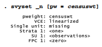
Any number of weight variables can exist in the same dataset, and svyset used repeatedly to select among them as needed for particular analysis. The weights affect analysis only when we apply them through svy: or other explicitly weighted commands. For the remainder of this chapter, we return to the Granite State Poll weighted by censuswt, a variable calculated by the UNH Survey Center to combine design weighting (for number of adults, and number of phone lines) with poststratification (for gender and region within New Hampshire).

Source: Hamilton Lawrence C. (2012), Statistics with STATA: Version 12, Cengage Learning; 8th edition.