Measurement and Structural Equation Models by using Stata

Chapter 8 took a first look at structural equation modeling, beginning with a regression-like example involving relationships among observed variables (Figure 8.15). Structural equation models can also incorporate measurement models, which resemble factor analysis. Measurement models posit one or more unobserved, factor-like latent variables that cause variation in observed variables. Figure 11.10 illustrates using the Pacific Northwest CERA survey.

. use C:\data\PNWsurvey2_11.dta, clear

Two unobserved, latent variables named Enviro and Resjobs appear in Figure 11.10. Their names intentionally echo those given to factor scores in the previous section, but for this analysis we are starting over. No variables by those names exist. In structural equation modeling, Stata (by default) follows a convention of representing latent variables with names that start with a capital letter. Latent variable Enviro is depicted as causing some of the variation in six observed variables, the same ones that loaded mainly on our factor 1 in the previous section. Latent variable Resjobs explains variation in four other observed variables which loaded mainly or in part on factor 2. Note the graphical conventions of oval outlines for latent variables and rectangular outlines for observed variables. A curved, double-headed arrow represents the non-causal correlation between Enviro and Resjobs.

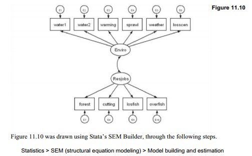
Select the Add measurement Component (M) tool from the left-hand margin, and place it at the location desired for a latent variable within the plot space. Give the latent variable a name starting with a capital letter, such as Enviro. Select Measurement variables to be explained by this latent variable by choosing their names from a list. Select a Measurement direction, such as Up. Click OK, then repeat for a second latent variable in a different location such as Resjobs, with Measurement direction … Down. Click OK again. Finally, use the Add covariance (C) tool from the right margin to place a curved, double-headed arrow for the correlation or covariance between the latent variables.

Figure 11.11 shows the same measurement model after estimation. Coefficients along the paths from latent to observed variables represent standardized regression coefficients analogous to factor loadings. Each observed variable also has its own unique variance, given by the e (epsilon) terms in this path model. Enviro and Resjobs have a correlation of .62.

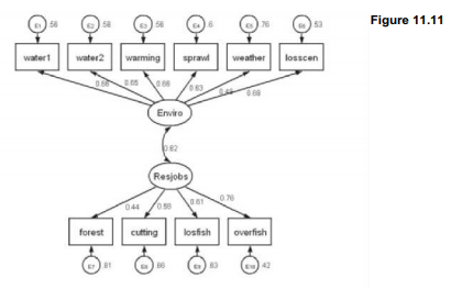
Once a path model such as Figure 11.10 has been drawn, simply clicking on Estimate will populate the graph with statistical results. Stata displays abundant information by default, but for some purposes, such as publication, we might want to keep things simple. Figure 11.11 contains only survey-weighted, standardized regression coefficients or variances, all in fixed display format with two digits right of the decimal. Simplifications were controlled through the following menu choices.

Settings > Variables > All … > Results > Exogenous variables > None > OK

Settings > Variables > All … > Results > Endogenous variables > None > OK

Settings > Variables > Error … > Results > Error std. variance > OK

Settings > Connections > Paths > Results > Std. parameter > OK

Settings > Connections > All > Results > Result 1 > Format %3.2f > OK > OK

Estimation > Estimate > Weights > Sampling weights … (select variable such as surveywt) > OK

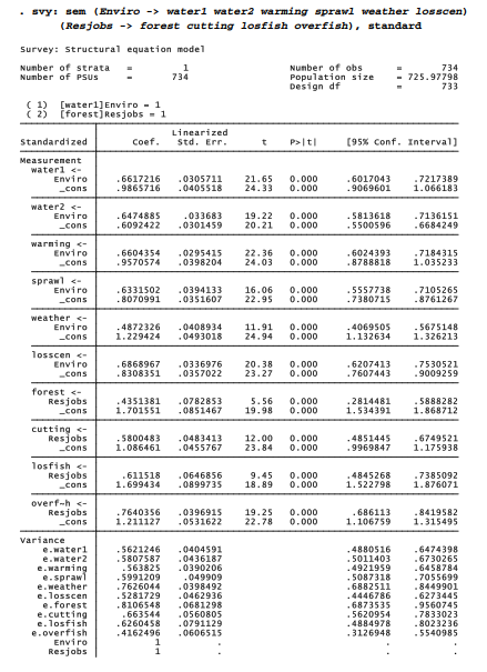
The same model can be estimated directly by a sem command, without going through the SEM Builder. In the command below, note the svy: prefix, which applies survey weighting to sem as it does to regress and many other Stata procedures. Standardized coefficients from this output correspond to the path coefficients in Figure 11.11. Unique variances of the observed variables, and the standardized covariance (i.e., correlation) between latent variables, likewise correspond to values shown in Figure 11.11.

Figure 11.12 shows an example that combines a measurement model (latent variable Enviro, explaining variation in the six observed variables water1 through losscen) with a regression model in which Enviro itself is explained by five observed background variables, age through newcomer. Conceptually, Figure 11.12 resembles our analysis in the previous section taking factor score enviro as a dependent variable regressed on age through newcomer. The structural equation approach formally combines aspects of factor analysis and regression into one model. It supports estimation and testing of a wide range of alternative specifications such as error correlations, and relationships involving other observed or latent variables.

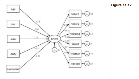
The following command estimates the same model seen in Figure 11.12, providing further detail.

. svy: sem (Enviro -> water1 water2 warming sprawl weather losscen)

(age sex educ party newcomer -> Enviro), standard

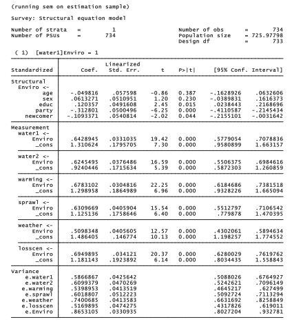
We find that educ,party and newcomer all have significant effects on the latent variable Enviro, whereas age and sex do not. These results agree with our previous regression of factor score enviro on the same five predictors.

The topic of structural equation modeling with Stata deserves at least one book of its own. The examples in this chapter, and those of Chapter 8, take only a first look. Stata’s Structural Equation Modeling Reference Manual includes a complete description of the commands, along with a library of 26 examples that take the reader much farther.

Source: Hamilton Lawrence C. (2012), Statistics with STATA: Version 12, Cengage Learning; 8th edition.