Recent Climate Change by using Stata

Shifting scale from thousands of years to only the past thirty, the rest of this chapter looks at how climate has changed recently. Dataset Climate.dta contains three time series estimating monthly global temperatures from 1980 through 2010, along with four possible drivers or causes of temperature. Two of the temperature indexes derive from surface-temperature measurements (NCDC and NASA), while a third independently estimates lower-troposphere temperatures from satellite data (UAH). See the Dataset Sources appendix for information about all of these variables, brought together from different sources.

The 1980-2010 time window covered by Climate.dta was constrained by available data: the global average CO₂ level time series used here begins in 1980, and the Aerosol Optical Depth data had been updated, at this writing, only through 2010. This file is tsset by myear, a monthly variable defined from separate month and year variables found in the original data sources. Internally, Stata defines monthly variables as the number of months since January 1960, just as it defines date variables as the number of days since January 1, 1960. Here myear has a %tmmCY format, so it will appear to us as Jan1980, Feb1980 and so forth. If not already done, creating this monthly time variable and tsseting the data would be necessary steps for later analysis.

. gen myear = ym(year, month)

. format myear %tmmCY

. label variable myear “Month, year”

. tsset myear

In a widely-cited paper, Foster and Rahmstorf (2011, building on earlier work by Lean and Rind, 2008) analyzed similar temperature and driver variables to uncover “the real global warming signal.” Their analysis is more thorough than the basic examples in this chapter. Nevertheless, we arrive at broadly similar conclusions.

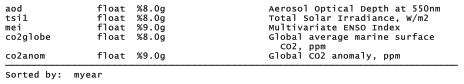
Figure 12.9 plots global temperature anomalies according to the National Climate Data Center (NCDC) index, ncdctemp. Temperature anomalies from an individual weather station represent deviations of observed temperature from the long-term mean temperature at that station for that month. Global temperature anomalies are subsequently calculated from a weighted average of many individual-station anomalies around the world. A gray line at zero marks the 20th-century mean.

. tsline ncdctemp, lw(medthick)

ytitle(“Global temperature anomaly vs. 1901’=char(150)’2000, ‘=char(176)’C”, size(medsmall))

yline(0, lcolor(gs12) lwidth(thick)) xtitle(“”)

xlabel(, grid gmin gmax)

All but two months in Figure 12.9 have temperatures above the 20th-century mean. The warming trend has been particularly steep since the mid-1970s, a period mostly captured by this graph. Its central high point is the globally hot month of February 1998, not surpassed (and then just barely) until January 2007. Both are more than two standard deviations higher than any month before 1980 in the NCDC data, which go back to 1880 (see Figure 2.1 in Chapter 2). However, warm temperatures through much of1998, together with cooler temperatures in some recent years, create a visual impression that global warming might have paused during the past decade. The final section of this chapter applies time series modeling to investigate possible explanations.

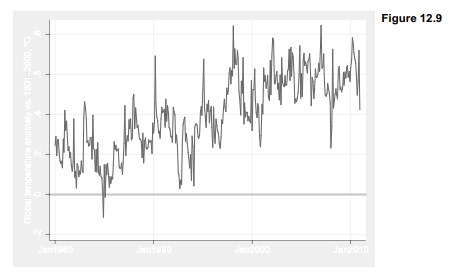
If systematic reasons exist, they might be found among the other variables in Climate.dta. These include four factors that physical scientists have identified as important drivers or causes of air temperature variations. Opaqueness of the atmosphere, here measured by Aerosol Optical Depth (AOD) at a wavelength of 550 nm, particularly reflects the influence of volcanic eruptions, which cool surface temperatures by injecting sunlight-blocking particles high into the atmosphere (Sato et al. 1993). Total Solar Irradiance (TSI) involves satellite-based measurements of the varying amounts of solar radiation (in Watts per square meter) received at the top of Earth’s atmosphere (Frohlich 2006). El Nino/Southern Oscillation (ENSO) events can substantially affect global air temperatures, either warming air through atmospheric changes that pool unusually warm surface water in the central and eastern tropical Pacific (El Nino), or cooling air temperatures by bringing more deep ocean water to the surface (La Nina). Some ENSO indicators are defined only from sea surface temperatures, creating circularity if then used to “explain” temperature in turn. This Multivariate ENSO Index (MEI), on the other hand, is defined from the first principal component of 6 variables observed over the tropical Pacific: sea-level pressure, zonal and meridional components of the surface wind, sea surface temperature, surface air temperature and total cloudiness fraction of the sky. MEI values substantially above zero indicate El Nino conditions, while values below zero indicate La Nina (Wolter and Timlin 1998). The fourth driver in these data is globally averaged marine-surface

carbon dioxide (CO₂) concentration in parts per million, based on measurements from a network of geographically dispersed sites (Masarie and Tans 1995). Variable co2globe gives the actual concentration, and co2anom crudely removes seasonal variations by subtracting from each value the 1980-2010 global mean for that month.

The last section of this chapter examines how well these four drivers together explain recent temperature change. Leading up to that analysis, the next sections present basic concepts and tools.

Source: Hamilton Lawrence C. (2012), Statistics with STATA: Version 12, Cengage Learning; 8th edition.