AMOS Functions Listed as Icons in Pinned Ribbon

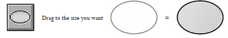
This function allows you to draw an observable variable.You can drag the square in the graph- ics window to the size of the box you want.

Example 3.1:

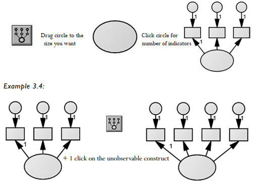
This function allows you to draw an unobservable variable.You can drag the circle in the graphics window to the size of the circle you want. Note: you will rarely need to use this function. AMOS provides a better option for drawing unobservable variables.

Example 3.2:

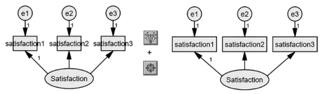
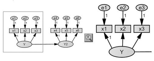
This function allows you draw an unobservable variable that includes indicators and error terms. This is the primary function you are going to use for drawing unobservable variables because it will include the indicators.You will initially draw/drag a circle to the size you want and then left- click on this circle to include an indicator. If you click twice on the unobservable (circle), AMOS will include two indicators.You can choose the number of indicators. If you have drawn the unob- servable construct and indicators but forgot to add an indicator, just select this function and click on the unobservable, and it will add another indicator.

Example 3.3:

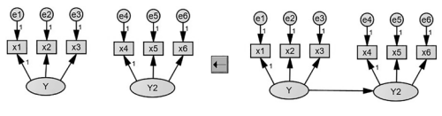
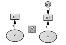
   This function lets you draw a path (parameter) between two objects in the graphics window.

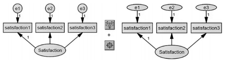
Example 3.5:

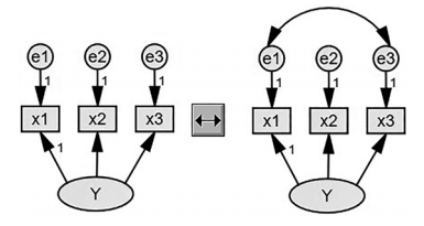
This function lets you draw a covariance. Note, if you drag this double headed arrow left to right, the arc of the line will be at the top. If you drag it right to left, the arc will be at the bot- tom. If you drag it top to bottom, the arc will be on the right. If you drag it from bottom to top, the arc of the line will be on the left.

Example 3.6:

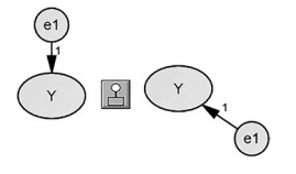
This function lets you add an error term to a variable. If a variable already has an error term added, then selecting this function and clicking on the variable again will rotate the error term.You can select the position you want the error term to be located.

Example 3.7:

Example 3.8:

This function will let you add a title to the graphics window.There is no real need for this unless you are printing your model or trying to share it with another person.

Example 3.9:

After clicking this function, you will get a pop-up window to enter a title along with position.

   This function will allow you see all the variables that have been labeled in the drawn model.

Example 3.10:

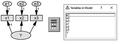
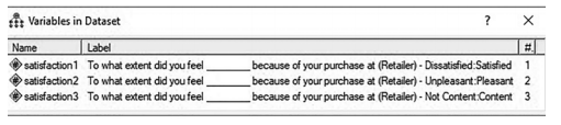
This function will show you all the variables that are listed in your data set. It will show the variable’s name, label, and the column number.

Example 3.11:

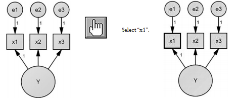
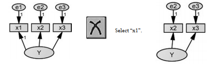
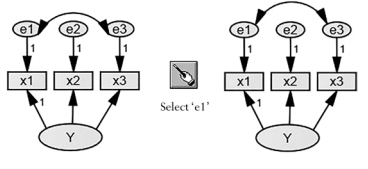
This function will allow you to select one object at a time.When you select an object, it will highlight it in blue.

Example 3.12:

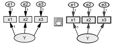
 This function will allow you to select every object that is on the graphics window.

Example 3.13:

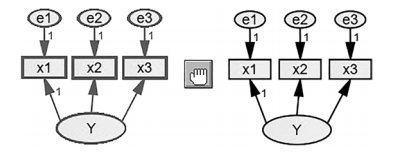
  This function will allow you to deselect all objects that are selected/highlighted.

Example 3.14:

This function will allow you to delete an object that is in the graphics window.

Example 3.15:

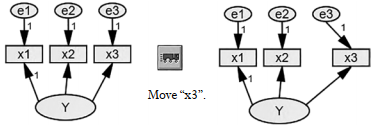
This function will allow you to move an object around the graphics window. If you select just this icon, you can move one object at time. If you want to move more than one object at a time, see the “preserve symmetries” function.

Example 3.16:

 

Example 3.17:

This function will create a duplicate of an object. If you choose this function and then select an object and drag, you will see a duplicate. This function will duplicate only one item at time unless the “preserve symmetries” button is selected, too. Note, the duplicate will have the same label, so this will need to be changed if it remains in the graphics window.

Example 3.18:

 

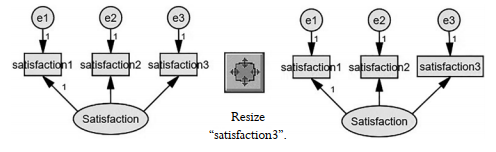
This function will allow you to change the shape of an object.You can change the height and width of an object.This is a handy function in order to see full variable names if they are bigger than the original object size.This function will let you resize only one object at time unless the “preserve symmetries” button is selected.

Example 3.19:

This is the preserve symmetries button which will allow you to change or move multiple objects within an unobservable construct that has indicators and error terms.This function is especially handy with the “move”, “resize”, and “copy” functions.

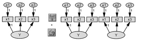
Example 3.20:

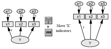
This will allow you to move all the “x” indicators at once instead of one at a time. You can space them out or move them in or out from the unobservable construct.

Example 3.21:

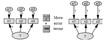
This will allow you to move all the error terms at once instead of one at a time. You can space them out or move them in or out from the indicators.

Example 3.22:

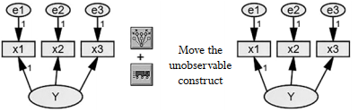
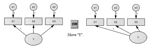
This will allow you to move the unobservable construct and all objects attached to it. In essence, this will move everything associated with the construct.

 Example 3.23:

With the preserve symmetries icon selected, you can resize numerous objects at once. If we were trying to resize the indicators, the boxes for all the indicators would resize to the desired size.

Example 3.24:

With the preserve symmetries icon selected, you can resize all the error terms at once instead of one at a time.

Example 3.25:

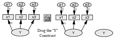
With the preserve symmetries icon selected, you can copy an unobservable and all its indicators. It makes a duplicate of the unobservable and all objects attached to it. Again, the labels are exactly the same in the duplicate, so you will need to change those if it is going to stay in the graphics window. This function is handy to use before the constructs have been labeled and you need another construct with the exact same number of indicators and error terms.

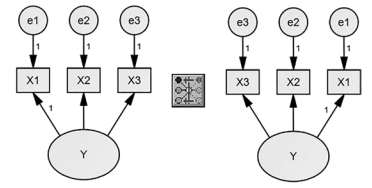
This function will allow you to rotate the indicators around the unobservable construct.

Example 3.26:

 

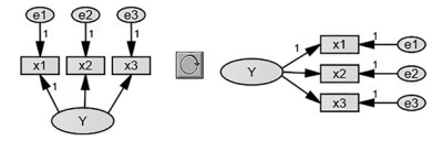
 This function will reflect the indicators of an unobserved construct. It is like a mirror function.

Example 3.27:

 

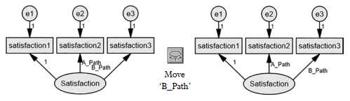
This function will allow you to move parameter labels so that you can see them clearly.

Example 3.28:

This is the touch up icon. It will rearrange paths and covariances to make them easier to see. It makes the paths and covariances pleasing to the eye from a graphical standpoint. Click the areas you want to clean up.

Example 3.29:

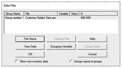
 This is the select data file function. This is where you will link the raw data to AMOS.

Example 3.30:

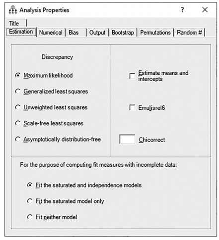
This is the Analysis Properties icon. This function will allow you to see numerous options for the output you want displayed after running the analysis. After clicking this icon, a pop-up window will appear.There are eight tabs at the top of the pop-up window that will allow you to choose different output options.

Example 3.31:

This is the calculate results icon.This is the icon you will select when you are ready to run your analysis.

This is the view output icon. Selecting this icon will take you to the text output after an analy- sis has been run.

This is the copy model to the clipboard icon. This will copy the model drawn on the graphics window to the clipboard for you to paste in another area or document.

This is the save current model icon. This will let you save your work.

This is the zoom on a specific area function. After selecting this icon, you can drag a box around a specific area and that selection will be zoomed in.

Example 3.32:

This is the zoom-in function. It will zoom the whole page on the graphics window in order for everything to become larger.

This is the zoom-out function. It will zoom out the whole page on the graphics window in order to see more of the page.

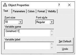
This is the Object Properties function. This is where you can change the properties of an object such as changing a variable name or label. You can also name and fix parameters. Another option available in this function is to change text size, style, and color scheme.There are five tabs at the top that will change different properties of an object.

Example 3.33:

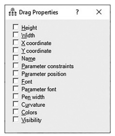
This is the drag properties function.This function will let you drag object properties to other objects in the graphics window. Note that the drag properties pop-up window has to be active for the “dragging” function to work across properties.You can drag an object’s properties to numerous objects if they are selected/highlighted first.

Example 3.34:

This is the reposition model function.This where you can scroll your model to the left and right and see more of what is on the graphics window.This is usually needed only if you have zoomed in on an area and need to see a subsequent area that is off the screen.

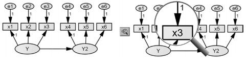
This is the examine diagram with loupe icon. This is just a big magnifying glass that lets you see in a desired area without zooming in.

Example 3.35:

This is the “zoom page” function.This function will magnify to view the whole page. Selecting this icon will either zoom in or out to let you see the whole page AMOS graphics is using.

This is the resize whole model to fit the page icon. This is where AMOS will resize the entire model to fit on the page. I would caution you not to use this option. It will force the model to the page in often weird and cramped ways.

This is the Bayesian Analysis function. Selecting this icon will take you to a pop-up window that will perform Bayesian analysis.

This is the multi-group analysis function. Choosing this icon will label parameters across groups and also suggest models to compare across groups.

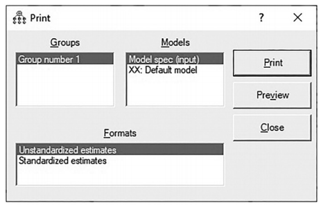
This is the print function.This icon will allow you to print the model on the graphics window. It will also allow you to print unstandardized and standardized estimates on the model. You can also choose between groups on the model you choose to print.

Example 3.36:

 This is the undo change function.

This is the redo change function.

This is the specification search function.This function lets you explore what the fit of a model is if you remove paths from the initial model.

Source: Thakkar, J.J. (2020). “Procedural Steps in Structural Equation Modelling”. In: Structural Equation Modelling. Studies in Systems, Decision and Control, vol 285. Springer, Singapore.