Problem 11.2: GLM Two-Factor Multivariate Analysis of Variance with SPSS

MANOVA is also useful when there is more than one independent variable and several related dependent variables. Let’s answer the following questions:

• Do students who differ in math grades and gender differ on a linear combination of two dependent variables (math achievement and visualization test)? Do males and females differ in terms of whether those with higher and lower math grades differ on these two variables (is there an interaction between math grades and gender)? What linear combination of the two dependent variables distinguishes these groups?

We already know the correlation between the two dependent variables is moderate (r = .42), so we will omit the correlation matrix. Follow these steps:

• Select Analyze → General Linear Model → Multivariate.
• Click on Reset.
• Move math achievement and visualization test into the Dependent Variables box (see 11.1 if you need help).
• Move both math grades and gender into the Fixed Factor(s)
• Click on Options.
• Check Descriptive statistics, Estimates of effect size, Observed power Parameter estimates, and Homogeneity tests (see 11.2).
• Click on Continue.
• Click on OK.

Compare your output with Output 11.2.

Output 11.2: Two-Way Multivariate Analysis of Variance

GLMmathach visual BY mathgr gender /METHOD = SSTYPE(3)

/INTERCEPT = INCLUDE

/PRINT = DESCRIPTIVE ETASQ OPOWER PARAMETER HOMOGENEITY

/CRITERIA = ALPHA(.05)

/DESIGN = mathgr gender mathgr*gender.

General Linear Model

Interpretation of Output 11.2

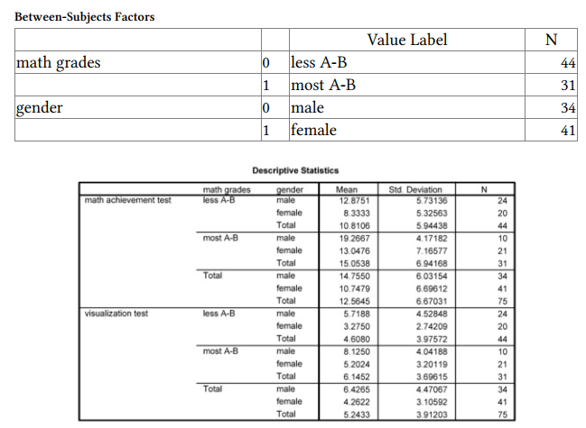
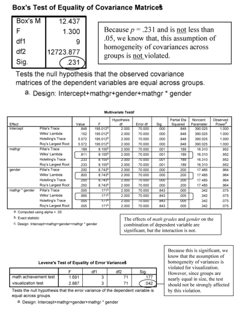
Many of the tables are similar to those in Output 11.1. For the Descriptive Statistics, we now see means and standard deviations of the dependent variables for the groups made up of every combination of the two levels of math grades and the two levels of gender. Box’s test again is not statistically significant, indicating that the assumption of homogeneity of

covariance matrices is met.

The main difference in 11.2, compared with 11.1b, for both the Multivariate Tests table and the univariate Tests of Between-Subjects Effects table, is the inclusion of two main effects (one for each independent variable) and one interaction (of math grades and gender; shown in the output as math grades * gender). The interpretation of this interaction, if it were statistically significant, would be similar to that in Output 11.1. However, note that although both the multivariate main effects of math grades and gender are statistically significant, the multivariate interaction is not statistically significant. Because the interaction was not statistically significant, we can look at the univariate tests of main effects, but we should not examine the univariate interaction effects.

Levene’s test indicates that there is heterogeneity of variances for visualization test. Again, we could have transformed that variable to equalize the variances. However, if we consider only the main effects of gender and of math grades (since the interaction is not statistically significant), then Ns are approximately equal for the groups (34 and 41 for gender and 31 and 44 for math grades), so this is less of a concern.

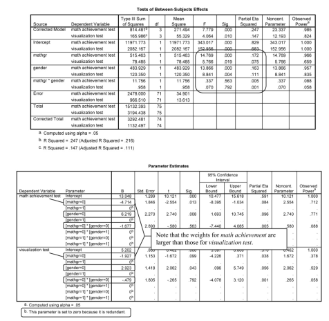
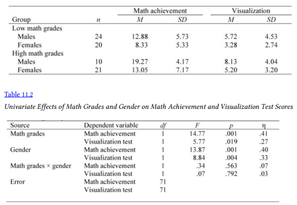
The Tests of Between-Subjects Effects table indicates that there are statistically significant main effects of both independent variables on both dependent variables, with medium to large effect sizes. For example, the “effect” of math grades on math achievement is large (eta = .41) and the effect of math grades on visualization test is medium (eta = .27). Refer again to Table 5.5. Note that both of these had relatively high power (.97 and .70, respectively).

The Parameter Estimates table now has three dummy variables: for the difference between students with less A-B and more A-B (MATHGR = 0), for male versus not male (GEND = 0), as well as for the interaction term (MATHGR = 0 GEND = 0). Thus, we can see that math achievement contributes more than visualization test to distinguishing students with better and worse math grades as well as contributing more to distinguishing boys from girls.

Example of How to Write About Output 11.2

Results

To assess whether boys and girls with higher and lower math grades have different math achievement and visualization test scores and whether there was an interaction between gender and math grades, a multivariate analysis of variance was conducted. (The assumptions of independence of observations and homogeneity of variance/covariance were checked and met. Bivariate scatterplots were checked for multivariate normality.) The interaction was not statistically significant, Wilks’ A = .995, F(2, 70) = .17, p =.843, multivariate n² = -005- The main effect for gender was statistically significant, Wilks’ A = .800, F(2, 70) = 8.74, p < .001, multivariate n² = -20- This indicates that the linear composite of math achievement and visualization test differs for males and females. The main effect for math grades is also statistically significant, Wilks’ A = .811, F(2, 70) = 8.15, p = .001, multivariate n² = .19. This indicates that the linear composite differs for different levels of math grades. Follow-up ANOVAs (Table 11.2) indicate that effects of both math grades and gender were statistically significant for both math achievement and visualization. Males scored higher on both outcomes and students with higher math grades were higher on both outcomes (see Table 11.1).

Source: Leech Nancy L. (2014), IBM SPSS for Intermediate Statistics, Routledge; 5th edition;

download Datasets and Materials.