Application 11: Addressing the Issues of Missing Data with AMOS

1. Key Concepts

• Unstructured versus structured missing data
• Basic patterns of missing data
• Ad hoc versus theory-based strategies for dealing with missing data
• Amos approach to dealing with missing data

Missing (i.e., incomplete) data, an almost inevitable occurrence in social science research, may be viewed either as a curse or as a gold mine of untapped resources. As with other life events, the extent to which they are viewed either positively, or negatively is a matter of perspective. For example, McArdle (1994) noted that, although the term, “missing data,” typically conjures up images of negative consequences and problems, such missingness can provide a wealth of information in its own right and, indeed, often serves as a useful part of experimental analyses. (For an interesting example in support of this statement, see Rosen, 1998.) Of import, is the extent to which and pattern by which data are missing, incomplete, or otherwise unobserved, and the steps that can be taken in addressing this situation.

Missing data can occur for a wide variety of reasons that are usually beyond the researcher’s control and, thus, missingness of this nature is termed unstructured missing data. Examples of unstructured missing data are as follows: absence on the day of data collection, failure to answer cer­tain items in the questionnaire, refusal to answer sensitive items related to one’s age and/or income, equipment failure or malfunction, attrition of subjects (e.g., family moved away, individual no longer wishes to partici­pate, subject dies), and the like.

In contrast, data may be missing by design, in which case the researcher is in total control. This type of missingness is termed structured missing data. Two examples suggested by Kline (1998) include the cases where (a) a questionnaire is excessively long and the researcher decides to administer only a subset of items to each of several different subsamples, and (b) a relatively inexpensive measure is administered to the entire sam­ple, whereas another more expensive test is administered to a smaller set of randomly selected subjects. Needless to say, there may be many more examples that are not cited here.

Because missing data can lead to inefficient analyses and seriously bias conclusions drawn from an empirical study (Horton & Kleinman, 2007), it is essential that they be addressed, regardless of the reason for their missingness. The extent to which such conclusions can be biased depends on both the amount and pattern of missing values. Unfortunately, to the best of my knowledge, there are currently no clear guidelines regarding what constitutes a “large” amount of missing data, although Kline (2011, p. 55) suggests that “a few missing values, such as less than 5% on a single variable, in a large sample may be of little concern.” He further states that this guideline is particularly so if the missing values occurred accidentally. That is, they are not of a systematic nature. On the other hand, guidelines related to the pattern of incomplete data are now widely cited and derive from the seminal works of Rubin (1976), Allison (1987), and Little and Rubin (1987). In order for you to more fully comprehend the Amos approach to handing incomplete data, I now review the differential patterns of missingness proposed by Rubin and by Little and Rubin.

2. Basic Patterns of Missing Data

Rubin (1976) and later Little and Rubin (1987) distinguished between three primary patterns of missing data: those missing completely at ran­dom (MCAR), those missing at random (MAR), and those considered to be nonignorable (i.e., systematic; NMAR). A brief description of each is now provided.

• MCAR represents the most restrictive assumption and argues that the missingness is independent of both the unobserved values and the observed values of all other variables in the data. Conceptualizing the MCAR condition from a different perspective, Enders (2001) sug­gests considering these unobserved values as representing a random subsample of the hypothetically complete data. Indeed, Muthen, Kaplan, and Hollis (1997) note that MCAR is typically what is meant when researchers use the expression, albeit imprecisely, “missing at random.”
• MAR is a somewhat less restrictive condition than MCAR and argues that the missingness is independent only of the missing values and not of the observed values of other variables in the data. That is to say, although the occurrence of the missing values, themselves, may be random, their missingness can be linked to the observed values of other variables in the data.
• NMAR is the least restrictive condition and refers to missingness that is nonrandom, or of a systematic nature. In other words, there is an existing dependency between the variables for which the values are missing and those for which the values are present. This condi­tion is particularly serious because (a) there is no known statistical means to alleviate the problem, and (b) it can seriously impede the generalizability of findings.

Of the three patterns of missingness, distinction between MCAR and MAR appears to be the most problematic. Indeed, Muthen et al. (1987) noted that most researchers, when confronted with incomplete data, typi­cally assume that the missingness is MCAR when, in fact, it is often MAR. To help you get a better grasp of the difference between these two pat­terns of missingness, let’s examine an ultra-simple example. Drawing on the works of Allison (1987) and Little and Rubin (1987), and paraphrasing Arbuckle (1996), suppose that a questionnaire is composed of two items. One item taps into years of schooling; the other taps into income. Suppose, further, that while all respondents answer the education question, not eve­ryone answers the income question. Within the framework of the miss­ingness issue, the question is whether the incomplete data on the income variable are MCAR or MAR. Rubin reasons that if a respondent’s answer to the income question is independent of both income and education, then the missing data can be regarded as MCAR. If, on the other hand, those with higher education are either more or less likely than others to reveal their income, but among those with the same level of education the probability of reporting income is unrelated to income, the missing data are MAR. Finally, given that, even among people with the same level of education, high-income individuals are either more or less likely to report their income, then the missing data are not even MAR; the systematic pattern of this type of missingness makes them NMAR (see Jamshidian & Bentler, 1999; Enders, 2001). (For an excellent explanation and illustra­tion of these three forms of missingness, readers are referred to Schafer & Graham, 2002; see also Graham & Coffman, 2012, for a slightly different approach in explaining these differences.)

Having identified the three types of missingness that can occur, of interest now are the strategies considered to be the most appropriate in addressing the problem. Graham and Coffman (2012) stress that, as with all statistical analyses, the primary goal in dealing with missing data is the use of methodologically sound strategies that will lead to unbiased esti­mates, appropriate standard errors or confidence intervals, and maximum statistical power. Over at least the past 15 years, a review of the SEM lit­erature has shown a surge of interest in developing newer approaches to addressing the issue of missing data. As a consequence, many, if not most of the earlier and very popular methods used are now no longer consid­ered to be optimal and are therefore not recommended (see, e.g., Graham & Coffman, 2012; Savalei & Bentler, 2009). However, because many of these older techniques continue to be used in dealing with missing data, I include them in the list of methodological approaches below by way of a caveat to researchers that these methods are no longer considered to be appropriate and therefore not recommended for a variety of reasons, as noted below.

3. Common Approaches to Handling Incomplete Data

Ad Hoc Approaches to Handling Missing Data (Not recommended)

The strategies included here are typically referred to as “ad hoc” or “indir­ect” methods in addressing the presence of missing data as they lack any kind of theoretical rationale. As noted above, these techniques are now considered to be outdated and “may do more harm than good, produ­cing answers that are biased, inefficient (lacking power), and unreliable” (Schafer & Graham, 2002, p. 147).

Listwise deletion. By far the most popular of the older methods for deal­ing with missing data is that of listwise deletion. Such popularity likely got its jumpstart in the 1980s when numerous articles appeared in the SEM literature detailing various problems that can occur when the analysis of covariance structures is based on incomplete data (see, e.g., Boomsma, 1985; Bentler & Chou, 1987). Because SEM models are based on the prem­ise that the covariance matrix follows a Wishart distribution (Brown, 1994; Joreskog, 1969), complete data are required for the probability density. In meeting this requirement, researchers have therefore sought to modify incomplete data sets, either through removal of cases or the substitution of values for those that are unobserved. The fact that listwise deletion of missing data is by far the fastest and simplest answer to the problem likely has led to the popularity of its use.

Implementation of listwise deletion simply means that all cases having a missing value for any of the variables in the data are excluded from all computations. As a consequence, the final sample to be used in the anal­yses includes only cases with complete records. The obvious disadvan­tage of the listwise deletion approach is the loss of information resulting from the reduced sample size. As a result, two related problems subse­quently emerge: (a) the decrease in statistical power (Raaijmakers, 1999), and (b) the risk of nonconvergent solutions, incorrect standard errors, and other difficulties encountered in SEM when sample sizes are small (see, e.g., Anderson & Gerbing, 1984; Boomsma, 1982; Marsh & Balla, 1994; Marsh, Balla, & McDonald, 1988). Of course, the extent to which these problems manifest themselves is a function of both the size of the original sample and the amount of incomplete data. For example, if only a few cases have missing values (e.g., less than 5%) and the sample size is adequately large, the deletion of these cases is much less problematic. However, Graham and Coffman (2012, p. 280) caution that a small amount of missingness on dif­ferent variables can add up to a meaningful loss of power due to the miss­ing cases. They note that it is in these types of cases that analysis of the complete data is a “poor alternative to using one of the recommended anal­ysis procedures.” Finally, use of listwise deletion assumes that the missing data are MCAR (Arbuckle, 1996; Brown, 1994; Graham & Coffman, 2012). Given the validity of this assumption, there will be consistent estimation of model parameters (Bollen, 1989a; Brown, 1994). However, failing such validity, the estimates will be severely biased, regardless of sample size (Graham & Coffman, 2012; Schafer & Graham, 2002).

Pairwise deletion. In the application of pairwise deletion, only cases having missing values on variables tagged for a particular computation are excluded from the analysis. In contrast to listwise deletion, then, a case is not totally deleted from the entire set of analyses, but rather, only from par­ticular analyses involving variables for which there are unobserved scores. The critical result of this approach is that the sample size necessarily varies across variables in the data set. This phenomenon subsequently leads to at least five major problems. First, the sample covariance matrix can fail to be nonpositive definite, thereby impeding the attainment of a convergent solution (Arbuckle, 1996; Bollen, 1989a; Brown, 1994; Graham & Coffman, 2012; Wothke, 1993, but see Marsh, 1998). Second, the choice of which sam­ple size to use in obtaining appropriate parameter estimates is equivocal (Bollen, 1989a; Brown, 1994). Third, goodness-of-fit indices, based on the X² statistic, can be substantially biased as a result of interaction between the percentage of missing data and the sample size (Marsh, 1998). Fourth, given that parameters are estimated from different sets of units, computa­tion of standard errors is problematic (Schafer & Graham, 2002; Graham & Coffman, 2012). Finally, consistent with listwise deletion of missing data, pairwise deletion assumes all missing values to be MCAR.

Single imputation. A third method for dealing with missing data is to simply impute or, in other words, replace the unobserved score with some estimated value. Typically, one of three strategies is used to provide these estimates. Probably the most common of these is Mean imputation, whereby the arithmetic mean is substituted for a missing value. Despite the relative simplicity of this procedure, however, it can be problematic in at least two ways. First, because the arithmetic mean represents the most likely score value for any variable, the variance of the variable will neces­sarily shrink; as a consequence, the correlation between the variable in question and other variables in the model will also be reduced (Brown, 1994). The overall net effect is that the standard errors will be biased, as will the other reported statistics. Second, if the mean imputation of miss­ing values is substantial, the frequency distribution of the imputed vari­able may be misleading because too many centrally located values will invoke a leptokurtic distribution (Rovine & Delaney, 1990). Third, Schafer and Graham (2002) note that mean substitution produces biased estimates under any type of missingness. In summary, Arbuckle and Wothke (1999) caution that, because structural equation modeling is based on variance and covariance information, “means imputation is not a recommended approach” (see also, Brown, 1994).

A second type of imputation is based on multiple regression proce­dures. With regression imputation, the incomplete data serve as the depend­ent variables, while the complete data serve as the predictors. In other words, cases having complete data are used to generate the regression equation that is subsequently used to postulate missing values for the cases having incomplete data. At least two difficulties have been linked to regression imputation. First, although this approach provides for greater variability than is the case with mean imputation, it nevertheless suffers from the same limitation of inappropriately restricting variance (Graham & Coffman, 2012). Second, substitution of the regression-predicted scores will spuriously inflate the covariances (Schafer & Olsen, 1998).

The third procedure for imputing values may be termed similar response pattern-matching (SRP-M) imputation. Although application of this approach is less common than the others noted above, it is included here because the SEM statistical package within which it is embedded is so widely used (LISREL 8; Joreskog & Sorbom, 1996a),¹ albeit this approach has no theoretical rationale (Enders & Bandalos, 2001). With SRP-M imputation, a missing variable is replaced with an observed score from another case in the data for which the response pattern across all variables is similar. If no case is found having compete data on a set of matching variables, no imputation is implemented (Byrne, 1998; Enders & Bandalos, 2001). As a consequence, the researcher is still left with a proportion of the data that is incomplete. In a simulation study of four missing-data SEM models (listwise deletion, pairwise deletion, SRP-M imputation, and full information maximum likelihood [FIML]), Enders and Bandalos (2001) reported the SRP-M approach to yield unbiased parameters for MCAR data, to show some evidence of biased estimates for MAR data, and, over­all, to be less efficient than the FIML approach.

Theory-based Approaches to Handling Missing Data (Recommended)

As noted earlier, there has been substantial interest on the part of statis­tical researchers to establish sound methodological approaches to dealing with missing data.

In a recent review of missing data issues within the context of SEM, Graham and Coffman (2012) categorized these updated strategies as model-based solutions and data-based solutions.

Model-based solutions. With the model-based solution, new statisti­cal algorithms are designed to handle the missing data and carry out the usual parameter estimation all in one step with no deletion of cases or imputation of missing values. Rather, this approach enables all cases to be partitioned into subsets comprising the same pattern of missing observa­tions (Kline, 2011). Importantly, this missing data approach in SEM is now more commonly termed the FIML solution (Graham & Coffman, 2012). Enders and Bandalos (2001) found the FIML technique to outperform the three other methods tested. Of import here is that FIML is the approach to missing data used in the Amos program which was one of the earliest SEM programs to do so.

Data-based solutions. This second recommended approach is based on a two-step process by which two data models are defined—one represent­ing the complete data and the other representing the incomplete data. Based on the full sample, the SEM program then computes estimates of the mean and variances such that they satisfy a statistical criterion (Kline, 2011). Methods in this category seek to replace the missing scores with estimated values based on a predictive distribution of scores that models the underlying pattern of missing data. As this book edition goes to press, two prominent methods here are the expectation-maximization (EM) solution and the multiple imputation (MI) solution. (For a comprehen­sive overview of EM, readers are referred to Enders, 2001a, and for MI, to Sinharay, Stern, & Russell, 2001.)

Of the two categories of theory-based approaches to missing-data han­dling described here, FIML and MI are the two techniques most generally recommended, as results from a number of simulation studies have con­sistently shown them to yield unbiased and efficient parameter estimates across a broader range of circumstances than was the case for the older set of techniques described earlier (Enders, 2008). (For a more extensive explanation and discussion of missing data as they bear on SEM analyses, readers are referred to Enders [2001a] and Schafer and Graham [2002]; for more details related to both model-based and data-based solutions, see Graham and Coffman [2012].)

Beyond this work, there is now a great deal of interest in resolving many problematic issues related to the conduct of SEM based on incom­plete data. The results of a sampling of these topics and their related schol­arly publications address the following array of concerns: (a) nonnormality (Enders, 2001b; Savalei, 2010; Savalei & Bentler, 2005; Yuan & Bentler, 2000; Yuan, Lambert, & Fouladi, 2004), and how it bears on longitudinal data (Shin, Davison, & Long, 2009); (b) evaluation of model goodness-of-fit (Davey, Savla, & Luo, 2005); (c) number of imputations needed to achieve an established statistical criterion (Bodner, 2008; Hershberger & Fisher, 2003; (d) use of FIML estimation with longitudinal models (Raykov, 2005) and use of MI versus FIML in multilevel models (Larsen, 2011); and (e) inclusion of auxiliary variables based on a two-stage approach (Savalei & Bentler, 2009), on FIML estimation (Enders, 2008), and on principal com­ponents analysis (Howard, Rhemtulla, & Little, 2015).

4. The Amos Approach to Handling Missing Data

Amos does not provide for the application of any of the older ad hoc (or indirect) methods described earlier (listwise and pairwise deletion; single imputation, etc.). Rather, the method used in Amos represents the theory-based full information maximum likelihood (FIML; direct) approach and, thus, is theoretically based (Arbuckle, 1996). Arbuckle (1996) has described the extent to which FIML estimation, in the presence of incomplete data, offers several important advantages over both the listwise and pairwise deletion approaches. First, where the unobserved values are MCAR, listwise and pairwise estimates are consistent, but not efficient (in the statistical sense); FIML estimates are both consistent and efficient. Second, where the unobserved values are only MAR, both listwise and pairwise estimates can be biased; FIML estimates are asymptotically unbiased. In fact, it has been suggested that FIML estimation will reduce bias even when the MAR condition is not completely satisfied (Muthen et al., 1987; Little & Rubin, 1989). Third, pairwise estimation, in contrast to FIML estimation, is unable to yield standard error estimates or to provide a method for testing hypotheses. Finally, when missing values are NMAR, all procedures can yield biased results. However, compared with the other options, FIML estimates will exhibit the least bias (Little & Rubin, 1989; Muthen et al., 1987; Schafer, 1997). (For more extensive discussion and illustration of the comparative advantages and disadvantages across the listwise, pairwise, and FIML approaches to incomplete data, see Arbuckle [1996] and Enders and Bandalos [2001].)

With this background on the major issues related to missing data, let’s move on to an actual application of FIML estimation of data that are incomplete.

5. Modeling with Amos Graphics

The basic strategy used by Amos in fitting structural equation models with missing data differs in at least two ways from the procedure followed when data are complete (Arbuckle & Wothke, 1999). First, in addition to fit­ting an hypothesized model, the program needs also to fit the completely saturated model in order to compute the x² value, as well as derived statis­tics such as the AIC and RMSEA; the independence model, as for complete data, must also be computed. Second, because substantially more computa­tions are required in the determination of parameter estimates when data are missing, the execution time can be longer (although my experience with the present application revealed this additional time to be minimal).

The Hypothesized Model

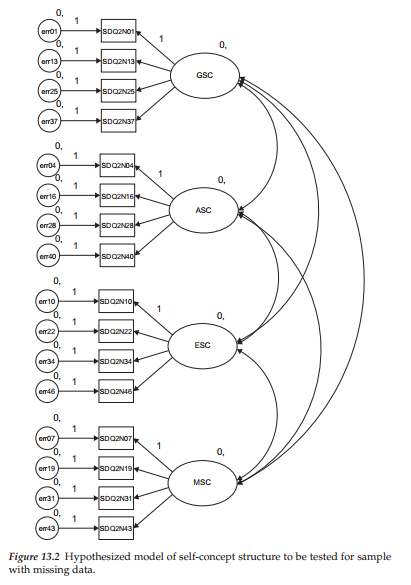
Because the primary interest in this application focuses on the extent to which estimates and goodness-of-fit indices vary between an analysis based on complete data and one for which the data are missing, I have chosen to use the same hypothesized CFA model as the one presented in Chapter 3. Thus, rather than reproduce the schematic representation of this model again here, readers are referred to Figure 3.1.

Although the same sample of 265 Grade 7 adolescents provides the base for both chapters, the data used in testing the hypothesized model in Chapter 3 were complete, whereas the data to be used in this chapter have 25% of the data points missing. These artificially derived missing data points were deleted randomly. Amos automatically recognizes miss­ing data designations from many different formats. In the case of the cur­rent data, which are in ASCII format with comma delimiters, two adjacent delimiters indicate missing data. In this case, then, two adjacent commas (,,) are indicative of missing data. For illustrative purposes, the first five lines of the incomplete data set used in the current chapter are shown here. SDQ2N01,SDQ2N13,SDQ2N25,SDQ2N37,SDQ2N04,

SDQ2N16,SDQ2N28,SDQ2N40,SDQ2N10,SDQ2N22,

SDQ2N34,SDQ2N46,SDQ2N07,SDQ2N19,SDQ2N31,SDQ2N43

• .3.4..6.2.6..5….6
• 6.6.6.5..6.6.6.6.6.6 4,6,6,2,6,4,6,3,6,5,4,5,6,6,3,1
• 6.3.5.6.6.6.5
• 3.4.4.4.4.6.5.6.3.4.4.5

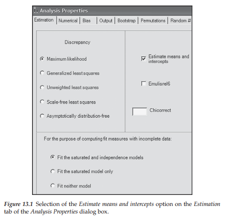
ML estimation of the hypothesized model incurs only one basic dif­ference when data are incomplete than when they are complete. That is, in specifying the model for analyses based on incomplete data, it is necessary to activate the Analysis Properties dialog box and then check off Estimate means and intercepts on the Estimation tab. Although this dialog box was illustrated in Chapter 8 with respect to structured means models, it is reproduced again here in Figure 13.1.

Once this input information has been specified, the originally hypoth­esized model shown in Figure 3.1 becomes transformed into the one shown in Figure 13.2. You will quickly recognize at least one similarity with the model shown in Figure 8.11 (but for the Low-track group) and the brief comparative display in Figure 8.12 with respect to the assignment of the 0. to each of the factors. Recall that these 0. values represent the latent factor means and indicate their constraint to zero. In both Figures 8.11 and 13.2, the means of the factors, as well as those for the error terms, are shown constrained to zero. Although the intercept terms were estimated for both the latent means model and the missing data model, their related labels do not appear in Figure 13.2. The reason for this important diffe­rence is twofold: (a) in testing for latent mean differences, the intercepts must be constrained equal across groups, and (b) in order to specify these constraints in Amos Graphics, it is necessary to attach matching labels to the constrained parameters. Because we are working with only a single group in this chapter, the intercept labels are not necessary.

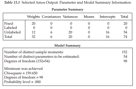
Selected Amos Output: Parameter and Model Summary Information

Presented in Table 13.1, you will see both the parameter summary and model summary information pertinent to our current incomplete data sam­ple. In the interest of pinpointing any differences between the incomplete and complete (see Table 3.3 and Figure 3.7) data samples, let’s now com­pare this information with respect to these same sections of the output file. First, notice that, although the number of fixed parameters in the model is the same (20) for the two samples, the number of unlabeled parameters (i.e., estimated parameters) varies, with the incomplete data group having 54, and the complete data sample having 38. The explanation of this discrep­ancy lies with the estimation of 16 intercepts for the incomplete data sample (but not for the complete data sample). Second, observe that although the number of degrees of freedom (98) remains the same across complete and incomplete data samples, its calculation is based upon a different number of sample moments (152 versus 136), as well as a different number of esti­mated parameters (54 versus 38). Finally, note that, despite the loss of 25% of the data for the one sample, the overall x² value remains relatively close to that for the complete data sample (159.650 versus 158.511).

Selected Amos Output: Parameter Estimates

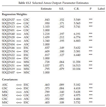
Let’s turn our attention now to a comparison of parameter estimates between the incomplete and complete data samples. In reviewing these estimates for the incomplete data sample (Table 13.2) and for the complete data sample (Table 3.4), you will see that the values are relatively close. Although the estimates for the incomplete data sample are sometimes a little higher but also a little lower than those for the complete data sample, overall, they are not very much different. Indeed, considering the substan­tial depletion of data for the sample used in this chapter, it seems quite amazing that the estimates are as close as they are!

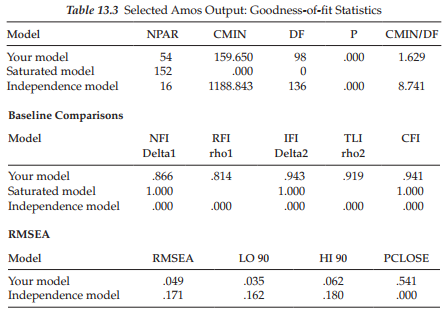
Selected Amos Output: Goodness-of-fit Statistics

In comparing the goodness-of-fit statistics in Table 13.3 for the incomplete data sample, with those reported in Table 3.5 for the complete data sam­ple, you will note some values that are almost the same (e.g., x² [as noted above]; RMSEA .049 versus .048), while others vary slightly at the sec­ond or third decimal point (e.g., CFI .941 versus .962). Generally speak­ing, however, the goodness-of-fit statistics are very similar across the two samples. Given the extent to which both the parameter estimates and the goodness-of-fit statistics are similar, despite the 25% data loss for one sam­ple, these findings provide strong supportive evidence for the effective­ness of the direct ML approach to addressing the problem of missing data values.

Source: Byrne Barbara M. (2016), Structural Equation Modeling with Amos: Basic Concepts, Applications, and Programming, Routledge; 3rd edition.