Chapter 2: Understanding the PLS-SEM Components

1. Inner (Structural) and Outer (Measurement) Models

Partial Least Squares Structural Equation Modeling (PLS-SEM) is a second-generation multivariate data analysis method that is often used in marketing research because it can test theoretically supported linear and additive causal models (Chin, 1996; Haenlein & Kaplan, 2004; Statsoft, 2013). With PLS-SEM, marketers can visually examine the relationships that exist among variables of interest in order to prioritize resources to better serve their customers. The fact that unobservable, hard-to-measure latent variables¹⁰ can be used in SEM makes it ideal for tackling business research problems.

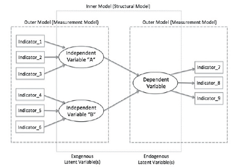
There are two sub-models in a structural equation model; the inner model¹¹ specifies the relationships between the independent and dependent latent variables, whereas the outer model¹² specifies the relationships between the latent variables and their observed indicators¹³ (see Figure 1). In SEM, a variable is either exogenous or endogenous. An exogenous variable has path arrows pointing outwards and none leading to it. Meanwhile, an endogenous variable¹⁴ has at least one path leading to it and represents the effects of other variable(s).

2. Determination of Sample Size in PLS-SEM

No matter which PLS-SEM software is being used, some general guidelines should be followed when performing PLS path modeling. This is particularly important, as PLS is still an emerging multivariate data analysis method, making it easy for researchers, academics, or even journal editors to let inaccurate applications of PLS-SEM go unnoticed. Determining the appropriate sample size is often the first headache faced by researchers.

In general, one has to consider the background of the model, the distributional characteristics of the data, the psychometric properties of variables, and the magnitude of their relationships when determining sample size. Hair et al. (2013) suggest that sample size can be driven by the following factors in a structural equation model design:

• The significance level
• The statistical power
• The minimum coefficient of determination (R2 values) used in the model
• The maximum number of arrows pointing at a latent variable

In practice, a typical marketing research study would have a significance level of 5%, a statistical power of 80%, and R² values of at least 0.25. Using such parameters, the minimum sample size required can be looked up from the guidelines suggested by Marcoulides & Saunders (2006), depending on the maximum number of arrows pointing at a latent variable as specified in the structural equation model (see Figure 2):

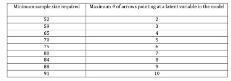
Figure 2: Suggested Sample Size in a Typical Marketing Research

Although PLS is well known for its capability of handling small sample sizes, it does not mean that your goal should be to merely fulfill the minimum sample size requirement. Prior research suggests that a sample size of 100 to 200 is usually a good starting point in carrying out path modeling (Hoyle, 1995). Please note that the required sample size will need to be increased if the research objective is to explore low-value factor intercorrelations with indicators that have poor quality.

3. Formative vs. Reflective Measurement Scale

There are two types of measurement scale in structural equation modeling; it can be formative or reflective.¹⁵

4. Formative Measurement Scale

If the indicators cause the latent variable and are not interchangeable among themselves, they are formative. In general, these formative indicators can have positive, negative, or even no correlations among each other (Haenlein & Kaplan, 2004; Petter et al., 2007). As such, there is no need to report indicator reliability, internal consistency reliability, and discriminant validity if a formative measurement scale is used. This is because outer loadings, composite reliability, and square root of average variance extracted (AVE) are meaningless for a latent variable made up of uncorrelated measures.

A good example of formative measurement scale is the measurement of employee’s stress level. Since it is a latent variable that is often difficult to measure directly, researchers have to look at indicators that can be measured, such as divorce, job loss, and car accidents. Here, it is obvious that a car accident does not necessarily have anything to do with divorce or job loss, and these indicators are not interchangeable.

When formative indicators exist in the model, the direction of the arrows has to be reversed. That is, the arrow should be pointing from the yellow-color formative indicators to the blue-color latent variable in SmartPLS. This can be done easily by right clicking on the latent variable and selecting “Invert measurement model” to change the arrow direction.¹⁶

5. Reflective Measurement Scale

If the indicators are highly correlated and interchangeable, they are reflective and their reliability and validity should be thoroughly examined (Haenlein & Kaplan, 2004; Hair et al., 2013; Petter et al., 2007). For example, in the next chapter, we will introduce you to a case study that is related to conducting survey in a restaurant. The latent variable Perceived Quality (QUAL) in our restaurant dataset is made up of three observed indicators¹⁷: food taste, server professionalism, and bill accuracy. Their outer loadings, composite reliability, AVE and its square root should be examined and reported.

In a reflective measurement scale, the causality direction is going from the blue-color latent variable to the yellow-color indicators. It is important to note that by default, SmartPLS assumes the indicators are reflective when the model is built, with arrows pointing away from the blue-color latent variable.¹⁸ One of the common mistakes that researchers make when using SmartPLS is forgetting to change the direction of the arrows when the indicators are formative instead of reflective. Since all of the indicators in this restaurant example are reflective, there is no need to change the arrow direction.

6. Should it be Formative or Reflective?

In case you are not 100% sure if a measurement model should be reflective or formative, the Confirmatory Tetrad Analysis (CTA-PLS) can be performed to find it out quantitatively. A step-by-step guide for using this technique is presented in the Chapter 6 of this book.

7. Guidelines for Correct PLS-SEM Application

In relation to other path modeling approaches, PLS-SEM is still relatively new to many researchers. Through extensive critical reviews of this methodology in the last several years, the academic community has developed some guidelines for correct PLS-SEM application. First of all, research should develop a model that is consistent with the theoretical knowledge currently available. As in other research projects, proper data screening should be performed to ensure accuracy of input. In order to determine the sample size necessary for adequate power (e.g., 0.8), the distributional characteristics of the data, the psychometric properties of variables, and the magnitude of the relationships between the variables have to be examined carefully.

Although PLS-SEM is well known for its ability to handle small sample sizes, that is not the case when moderately non-normal data are used, even if the model includes highly reliable indicators. As a result, researchers are strongly advised to check the magnitude of the standard errors of the estimates and calculate the confidence intervals for the population parameters of interest. If large standard errors and wide confidence intervals are observed, they are good indications that the sample size is not large enough for proper analysis. Prior research has indicated that a sample size of 100 to 200 is a good start in carrying out PLS procedures. The required sample size will further increase if you are examining low-value-factor intercorrelations with poor quality indicators.

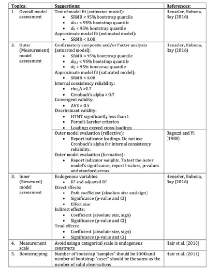
PLS is still considered by many as an emerging multivariate data analysis method, and researchers are still exploring the best practices of PLS-SEM. Even so, some general guidelines have been suggested in the literature. Figure 3 displays some of guidelines that should be considered.

Source: Ken Kwong-Kay Wong (2019), Mastering Partial Least Squares Structural Equation Modeling (Pls-Sem) with Smartpls in 38 Hours, iUniverse.