Chapter 12: New Techniques in PLS-SEM

1. Estimating Factor Models Using Consistent PLS (PLSc)

The traditional PLS algorithm has its shortcomings. Dijkstra & Schermelleh-Engel (2014) argue that it overestimates the loadings in absolute value and underestimates multiple and bivariate correlations between latent variables. It is also found that the R² value of endogenous latent variables is often underestimated (Dijkstra, 2010).

Building on Nunnally’s (1978) famous correction for attenuation formula, the Consistent PLS (PLSc) is proposed to correct reflective constructs’ correlations to make estimation results consistent with a factor-model (Dijkstra 2010; Dijkstra 2014; Dijkstra and Henseler 2015a; Dijkstra and Schermelleh-Engel 2014). In SmartPLS v3, the developers have added “Consistent PLS Algorithm” and “Consistent PLS Bootstrapping” to account for the correlations among reflective factors (see Figure 99).

The original PLS Algorithm and Bootstrapping functions are still available in the software. Which to choose depends on whether the researcher’s model has reflective or formative constructs:

If all constructs are reflective: use Consistent PLS Algorithm and Bootstrapping
If all constructs are formative: use PLS Algorithm and Bootstrapping (the original one)
If there is a mixture of reflective and formative constructs: use Consistent PLS Algorithm and Bootstrapping

In other words, if the constructs are modeled as factors, the researcher should use consistent PLS (PLSc) instead of traditional PLS with Mode A. There are also other considerations when using PLSc. For example, if a researcher’s model utilizes a higher-order construct, he or she should just use the two-stage approach and not the repeated indicator approach as the latter does not work well with PLSc. Also, if there is a huge discrepancy between the traditional PLS and PLSc results, the researcher should rethink if all reflective constructs truly follow a common factor model, or if they should use a composite (formative) model instead.

2. Assessing Discriminant Validity Using Heterotrait-Monotrait Ratio of Correlations (HTMT)

In PLS-SEM where there are reflective constructs, it is important to assess discriminant validity when analyzing relationships between latent variables. Discriminant validity needs to be established in order to confirm that the hypothesized structural paths results are real and not the result of statistical discrepancies.

The classical approach in assessing discriminant validity relies on examining (i) the Fornell-Larcker criterion, and
(ii) partial cross-loadings. This information is still available in the result report of SmartPLS v3. However, Henseler, Ringle and Sarstedt (2015) argued that these approaches cannot reliably detect the lack of discriminant validity in most research scenarios. They proposed an alternative approach called Heterotrait-monotrait ratio of correlations (HTMT) which is based on the multitrait-multimethod matrix.

3. HTMT Procedures

Let us use the “cafe100” dataset to illustrate how HTMT can be performed to check discriminant validity.
Go to the “Calculate” menu and select “Consistent PLS Algorithm”.
Under the “Setup” tab, check “Connect all LVs for Initial Calculation” and then press the “Start Calculation” button.
Once the algorithm converged, go to the “Quality Criteria” section and click the “Discriminant Validity” hyperlink.
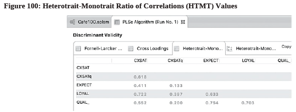
Go to the 3^rd tab where it says “Heterotrait-Monotrait Ratio (HTMT)” (see Figure 100).
Check the values. Since the maximum value 0.754 is below the 0.85 thresholds (i.e., the most conservative HTMT value), we say that discriminant validity is established in the model.
The next step is to assess HTMT inference criterion. To do that, first go back to the colorful model tab. Then, go to the “Calculate” menu and select “Consistent PLS Bootstrapping”.
On the 2^nd tab “Bootstrapping”, choose “Complete Bootstrapping” in the “Amount of Results” selection. This is an important step or else HTMT info will not be displayed.
Click the “Start Calculation” button to perform the bootstrapping procedure.
Once the result report opens, go to “Quality Criteria” and click the “Heterotrait-Monotrait Ratio (HTMT)” hyperlink. You may need to scroll down in order to view this link at the bottom of the screen.
Go to the 2^nd tab “Confidence Intervals Bias Corrected” to check the values (see Figure 101).

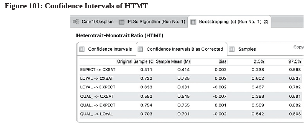
Look at the CI low (2.5%) and CI Up (97.5%) columns. Since all HTMT are significantly different from 1, discriminant validity is said to be established between these reflective constructs.

4. Contrasting Total Effects Using Importance-Performance Matrix Analysis (IPMA)

SmartPLS v3 has introduced a new way of reporting PLS-SEM results — The importance-performance matrix analysis (IPMA). It is often used in evaluating the performance of key business success drivers. IPMA is basically a xy-plot where the x-axis shows the “Importance” (Total Effect) of business success drivers using a scale of 0 to 1, and the y-axis shows the “Performance” of business success drivers using a scale of 0 to 100. This way, researchers can identify those predecessor constructs that have a strong total effect (high importance) but low average latent variable scores (low performance) for subsequent operational improvement.

IPMA requires the use of a metric scale or equidistant scale (with balanced positive and negative categories with a neutral category in the middle). Hence, indicators being measured on a nominal scale cannot utilize IPMA.

5. IPMA Procedures

Let us use the “cafe100” dataset to illustrate IPMA.
Run PLS Algorithm by going to the “Calculate” menu and select “Consistent PLS Algorithm”
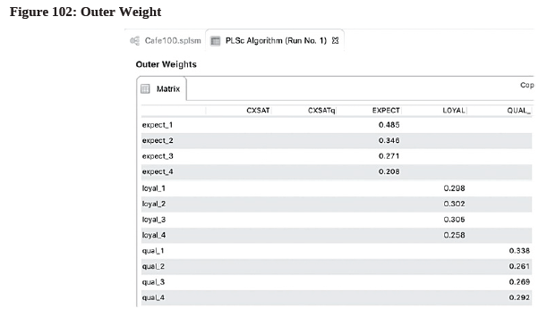
On the Results Report, check the signs of the outer weight to see if they are positive or negative by going to “Final Results Outer Weights”. In general, we want positive values. If there are any indicators having negative values (e.g., those larger than-0.1), they should be removed prior to running IPMA. In our case, all values are positive (see Figure 102), so we can proceed with IPMA.

Go back to the colorful model tab, then select “Importance-Performance Map Analysis (IPMA)” in the “Calculate” menu.
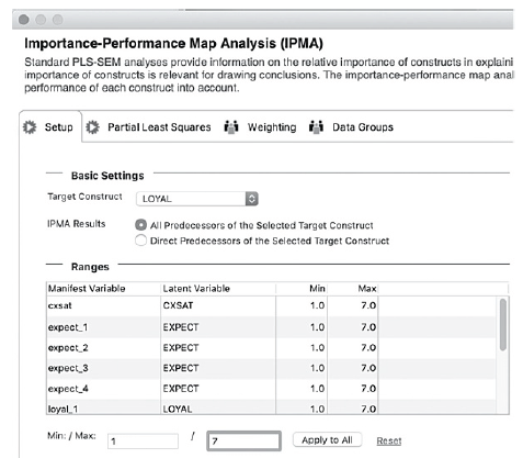
Specify the target construct LOYAL in the “Setup” tab, and choose the “All Predecessors of the Selected Target Construct” option. Also, enter the min or max value of the scale and press the “Apply to All” button. Once it’s all done, press the “Start Calculation” button (see Figure 103).
To view IPMA result graphically, go to “Quality Criteria 9 Importance-Performance Map [LOYAL] (constructs, unstandardized effects)” on the Results Page (see Figure 104).

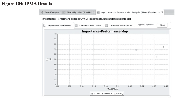
As shown in Figure 104, QUAL has a high total effect (i.e., high importance) but low performance in driving customer loyalty, so this is an area that the cafe owner should not be ignored for improvement once she has addressed the EXPECT items.

6. Testing Goodness of Model Fit (GoF) Using SRMR, d_ULS. and _dG

Prior to the development of Consistent PLS (PLSc), there was an established view that PLS-SEM could not be assessed globally for the overall model because it did not optimize any global scalar function (Henseler, Hubona and Ray, 2016). For years, it has been argued that the overall goodness-of-fit (GoF) cannot reliably distinguish valid from invalid models in PLS-SEM so this kind of assessment is rarely used and reported.

However, testing GoF as a way to contrast models is now possible under PLSc since it is a full-blown SEM method that provides consistent estimates for both factor and composite models. Researchers can now assess GoF within PLSc to determine whether a model is well-fitted or ill-fitted (Henseler et al, 2014), and to detect measurement model misspecification and structural model misspecification (Dijkstra and Henseler, 2014). Specifically, we want to understand the discrepancy between the “observed”¹¹⁰ or “approximated”¹¹¹ values of the dependent variables and the values predicted by the PLS model.

There are 3 different approaches to assess the model’s goodness-of-fit (Henseler et al, 2016):

Approximate fit criterion: The standardized root mean squared residual (SRMR)¹¹²

The lower the SRMR, the better the model’s fit. Perfect fit is obtained when SRMR is zero. SRMR value of 0.08 or lower is acceptable. A value significantly larger than 0.08 suggests the absence of fit.¹¹³

Exact fit criterion: The unweighted least squares discrepancy (d_ULS)

The lower the d_ULS, the better the model’s fit.

Exact fit criterion: The geodesic discrepancy (d_G)

The lower the d_G, the better the model’s fit.

7. GoF Procedures

Let us use the “cafe100” dataset to illustrate how GoF can be assessed.
Go to the “Calculate” menu and select “Consistent PLS Algorithm”.
Under the “Setup” tab, check “Connect all LVs for Initial Calculation” and then press the “Start Calculation” button.
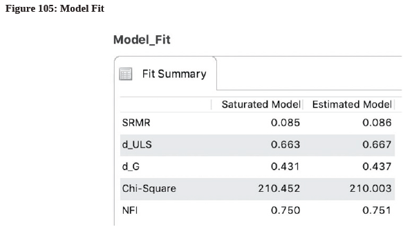
Once the algorithm converged, go to the “Quality Criteria” section and click the “Model Fit” hyperlink. The result is displayed in Figure 105.
Under the “Estimated Model” column, you can now find the values for SRMR, d_ULS, and d_G. for assessment using the guidelines as shown earlier in this section. In our model, we have an SRMR value of 0.086, which is slightly above the 0.08 threshold; this suggests a poor theoretical model fit.

Source: Ken Kwong-Kay Wong (2019), Mastering Partial Least Squares Structural Equation Modeling (Pls-Sem) with Smartpls in 38 Hours, iUniverse.