Chapter 3: Using SmartPLS Software for Path Model Estimation

1. Introduction to the SmartPLS Software Application

There are currently different versions of SmartPLS in circulation. The previous version, 2.0M3, is a freeware that has all of the core functionalities for PLS-SEM. Although it is only available on the Windows platform, this freely available version 2 is still used by thousands of researchers around the world because it does not have any limitation on the dataset. Once activated, this software has to be renewed online every three months with a free software license key that is e-mailed by the SmartPLS team to the registered user.

The current release of SmartPLS is 3.2.8 (as of February 2019), it is compatible with both Windows and macOS platforms. As compared to version 2, it adds many new and exciting functionalities such as Confirmatory Tetrad Analysis (CTA-PLS), Quadratic Effect Modeling (QEM), Measurement Invariance of the Composite Models (MICOM), Permutation Test, Finite Mixture Partial Least Squares (FIMIX-PLS), PLS Prediction-oriented Segmentation (PLS-POS), Consistent PLS (PLSc), Heterotrait-Monotrait Ratio of Correlations (HTMT), Importance-Performance Matrix Analysis (IPMA), and Goodness of Model Fit (GoF): SRMR, d_ULS, and d_G testing procedures.

Version 3 has a free “Student” version and also a paid “Professional/Enterprise” version. The student edition allows a maximum of 100 observations (rows) in the dataset and has limited algorithms and data export options as compared to the paid version.

2. Downloading and Installing the Software

To download SmartPLS version 2, please first go to https://www.smartpls.com/smartpls2 to fill out a product registration form. An e-mail from the SmartPLS team will then be sent to the user with the download link together with a software license key. Again, this release only supports the Windows platform. Intel-based Apple Mac users who want to use version 2 should utilize visualization software¹⁹ or Apple’s own Bootcamp function to run SmartPLS under the Windows OS environment²⁰.

To download SmartPLS version 3, please go to https://www.smartpls.com/downloads. Microsoft Windows user should can choose to download either the “32-bit Installer” or the “64-bit Installer”, depending on the user’s computer system configuration. For Mac users, there are two pieces of software to download: (i) DMG Installer for SmartPLS and (ii) Java Runtime.

If you are an instructor trying to teach PLS-SEM using SmartPLS 3, please ask students to download the software at home or campus prior to attending your lecture. This software is over 60MB in file size and it can be slow to download if all students are trying to access the server at the same time.

3. Solving Software Installation Problem on Recent Macs

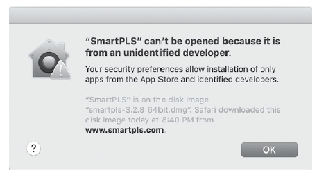
Most of my students who used the latest Macs (with macOS El Capitan 10.11, Sierra 10.12, High Sierra 10.13, or Mojave 10.14) have reported problems installing the SmartPLS software. After some investigations, it turned out that they either forgot to install the Java Runtime software as mentioned before or did not grant security permission for such software installation (see Figure 4).

To solve the permission problem, first go to the Apple menu and select “System Preferences…” Then, click the “Security & Privacy” icon and go to the “General” tab. Press the “Open Anyway” button where it says “SmartPLS” was blocked from opening because it is not from an identified developer (see Figure 5).

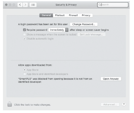
Figure 5: Security & Privacy Settings

A pop-up window will appear to ask if you are sure that you want to open this SmartPLS software. Click the “Open” button to complete the installation process.

4. Case Study: Customer Survey in a Restaurant (B2C)

The following customer satisfaction example will be used to demonstrate how to use the SmartPLS software application.

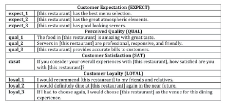
Customer satisfaction is an example of a latent variable that is multidimensional and difficult to observe directly. However, one can measure it indirectly with a set of measurable indicators²¹ that serve as proxy²². To understand customer satisfaction, a survey can be conducted to ask restaurant patrons about their dining experience. In this fictitious survey example, restaurant patrons are asked to rate their experience on a scale representing four latent variables, namely Customer Expectation (EXPECT), Perceived Quality (QUAL), Customer Satisfaction (SAT), and Customer Loyalty (LOYAL), using a 7-point Likert scales²³ [(1) strongly disagree, (2) disagree, (3) somewhat disagree, (4) neither agree nor disagree, (5) somewhat agree, (6) agree, and (7) strongly agree]. The conceptual framework is visually shown in Figure 6, and the survey questions asked are presented in Figure 7. Other than Customer Satisfaction (SAT) that is measured by one question, all other variables (QUAL, EXPECT, & LOYAL) are each measured by three questions. This design is in line with similar researches conducted for the retail industry (Hair et al., 2013).

Figure 6: Conceptual Framework – Restaurant Example

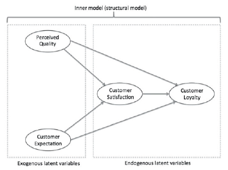
Figure 7: Questions for Indicator Variables

5. Data Preparation for SmartPLS

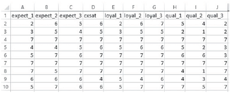
In this restaurant example, the survey data were manually typed into Microsoft Excel and saved as .xlsx format (see Figure 8). This dataset has a sample size of 400 without any missing values, invalid observations or outliers. To ensure SmartPLS can import the Excel data properly, the names of those indicators (e.g., expect_1, expect 2, expect_3) should be placed in the first row of an Excel spreadsheet, and no “string” value (e.g., words or single dot²⁴) should be used in other cells.

Figure 8 – Dataset from the Restaurant Example

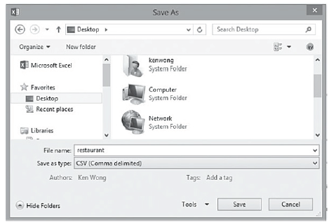
Since SmartPLS cannot take native Excel file format directly, the dataset has to be converted into .csv file format²⁵. To do this, go to the “File” menu in Excel, and choose “CSV (Comma Delimited)” as the file format type to save it onto your computer (see Figure 9).

6. Project Creation in SmartPLS

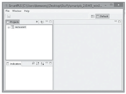
Now, launch the SmartPLS program and go to the “File” menu to create a new project. We will name this project as “restaurant” and then import the indicator data. Since there is no missing value²⁶ in this restaurant data set, we can press the “Finish” button to create the PLS file. Once the data set is loaded properly into SmartPLS, click the little “+” sign next to restaurant to open up the data in the “Projects” tab (see Figure 10).

Figure 10: Project Selection

Under the “restaurant” project directory, a “restaurant.splsm” PLS file and a corresponding “restaurant.csv” data file are displayed²⁷. Click on the first one to view the manifest variables under the “Indicators” tab (see Figure 11).

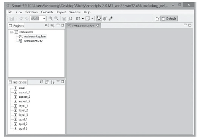
Figure 11: List of Indicators

7. Building the Inner Models

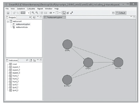
Based on the conceptual framework that has been designed earlier in this book (see Figure 6), an inner model can be built easily in SmartPLS by first clicking on the modeling window on the right-hand side, and then selecting the 2^nd last blue-color circle icon titled “Switch to Insertion Mode”. Click in the window to create those red-color circles that represent your latent variables. Once the circles are placed, right click on each latent variable to change the default name into the appropriate variable name in your model. Press the last icon titled “Switch to Connection Mode” to draw the arrows to connect the variables together (see Figure 12).

Figure 12: Building the Inner Model

8. Building the Outer Model

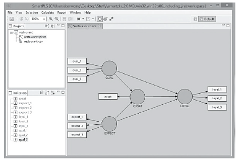
The next step is to build the outer model. To do this, link the indicators to the latent variable by dragging them one-by-one from the “Indicators” tab to the corresponding red circle. Each indicator is represented by a yellow rectangle, and the color of the latent variable will change from red to blue when the linkage is established. The indicators can be easily relocated on the screen by using the “Align Top/Bottom/Left/Right” function, if you right click on the blue-color latent variable. The resulting model should look like those in Figure 13.

Figure 13: Building the Outer Model

9. Running the Path-Modeling Estimation

Once the indicators and latent variables are linked together successfully in SmartPLS (i.e., no more red-color circles and arrows), the path modeling procedure can be carried out by going to the “Calculate” menu and selecting “PLS Algorithm”²⁸. If the menu is dimmed, just click on the main modeling window to activate it. A pop-up window will be displayed to show the default settings. Since there is no missing value²⁹ for our data set, we proceed directly to the bottom half of the pop-up window to configure the “PLS Algorithm – Settings” with the following parameters (see Figure 14):

• Weighting Scheme: Path Weighting Scheme
• Data Metric: Mean 0, Variance 1
• Maximum Iterations: 300
• Abort Criterion: 1.0E-5
• Initial Weights: 1.0

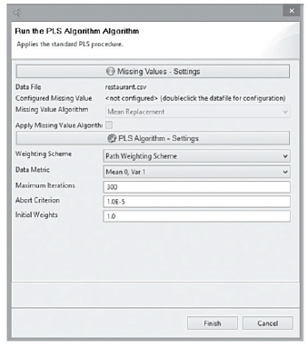
To run the path modeling, press the “Finish” button. There should be no error messages popping up on the screen, and the result can now be assessed and reported.

Source: Ken Kwong-Kay Wong (2019), Mastering Partial Least Squares Structural Equation Modeling (Pls-Sem) with Smartpls in 38 Hours, iUniverse.