Chapter 7: Handling Non-Linear Relationship Using Quadratic Effect Modeling (QEM)

1. Non-linear Relationship Explained

Experienced researchers would agree that variables do not always hold a linear relationship as in a straight line (Hay & Morris, 1991; Eisenbeiss, CorneliEen, Backhaus, & Hoyer, 2014). For example, in the field of marketing, advertising activities and sales revenue often hold a non-linear, quadratic relationship.⁴⁸ Consumers may be eager to buy a firm’s product or service after watching an attractive advertisement, but their intentions to make such purchases gradually drop after initial excitement is gone, even if they are being exposed to the advertisements continuously. In other words, the effect of advertising on sales gradually diminishes even though they have a positive relationship overall.

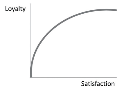
The same can be said for the relationship between customer satisfaction and loyalty. Although customer satisfaction (CXSAT) is usually affecting loyalty (LOYAL) in a positive way, they do not necessarily dictate a straight linear relationship all the time. In reality, customer satisfaction and loyalty often hold a non-linear, quadratic relationship. It is not uncommon to see customer’s loyalty towards a brand peaked out after a period of time even when they are still highly satisfied with the product or service. If we draw a graph, this relationship can be represented by a concave downward curve with a positive slope (see Figure 33).

Technically speaking, the non-linear relationship can be viewed as a linear relationship that is moderated by a newly created quadratic term (variable) that is a self-interaction of the exogenous construct (e.g., CXSAT * CXSAT).

To determine whether the variable of interest is having a linear or non-linear relationship, one should assess the following 2 aspects in PLS-SEM:

1. The significance of the quadratic term
2. The f² effect size of the quadratic term

2. QEM Procedures

1. Let us use the “cafe100” dataset for illustration. Assuming that we suspect a non-linear relationship exists between customer satisfaction (CXSAT) and customer loyalty (LOYAL), we can run Quadratic Effect Modeling (QEM) to see if that is the case.
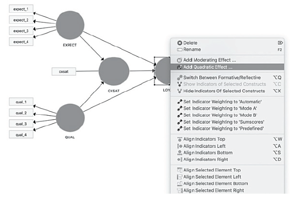
2. First, we need to create a quadratic term in the “Cafe100.splsm” tab. In our colorful model, right-click on the dependent variable (e.g., LOYAL) and choose “Add Quadratic Effect…”. (see Figure 34).

3. Select the independent variable “CXSAT” and set Calculation Method as “Two Stage” (see Figure 35). Use the other default settings. Click the “OK” button to build that Quadratic term.

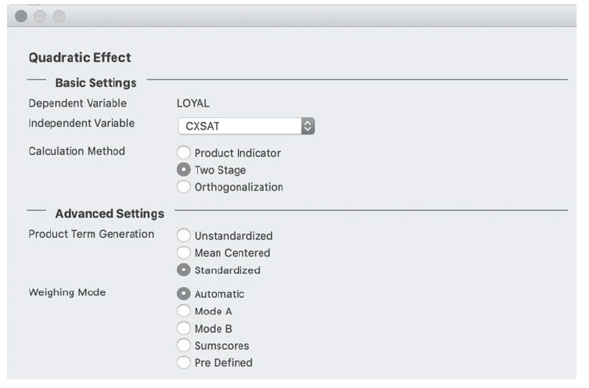
Figure 35: Quadratic Effect Settings

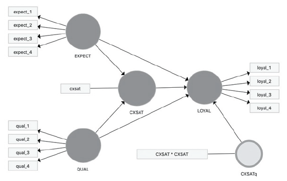
4. Rename the newly created quadratic term from “Quadratic Effect 1” to “CXSATq”. Right click on it and select “Show Indicators of Selected Constructs” (see Figure 36).

Figure 36: Renaming the Quadratic Term

5. Go to the “Calculate” menu and select “PLS Algorithm”. Run the estimation to obtain the path coefficients (see Figure 37).

Figure 37: PLS Algorithm Results

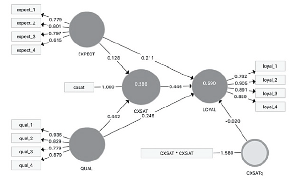
The following equation illustrates the results of the relationship between CXSAT and LOYAL:

LOYAL = 0.446 * CXSAT – 0.020 * CXSATq

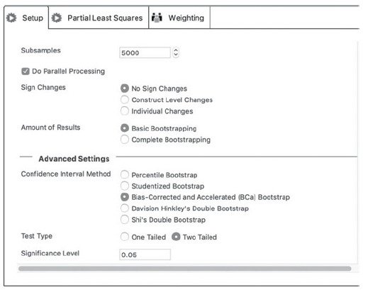
6. The significance of the quadratic term can then be determined using the “Bootstrapping” procedure. Go to the “Calculate” menu to select “Bootstrapping”. Run it using a subsample of 5000 (see Figure 38):

Figure 38: Bootstrapping

7. Once bootstrapping is completed, look at the “Mean, STDEV, T-Values, P-Value” tab in the Path Coefficients report. Check the corresponding p-value using the following hypotheses and a significance level of 0.05 (see Figure 39):

H_a: Satisfaction and Loyalty have significant non-linear, quadratic effect.

H_o: Satisfaction and Loyalty have insignificant non-linear, quadratic effect.

Figure 39: P-Values for the Quadratic Term Linkage

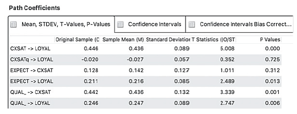
8. From Figure 35, it can be seen that in the CXSATq -> LOYAL row, the resulting P-Value is 0.725, which is larger than our significance level of 0.05. As a result, we accept the null hypothesis that Customer Satisfaction (CXSAT) and Loyalty (LOYAL) do not hold any significant non-linear, quadratic effect.
9. To confirm, we can double check the “Confidence Intervals Bias Corrected” tab (see Figure 40):

Figure 40: 95% Bias Corrected Confidence Interval

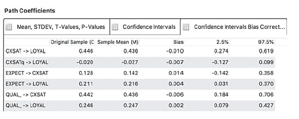
In the CXSATq – LOYAL row, the value zero falls in between the lower bound of-0.127 and upper bound of 0.099. Based on the 95% bias-corrected confidence interval, it can be concluded once again that CXSAT’s non­linear, quadratic effect on LOYAL is insignificant.

10. Other than assessing the significance of the quadratic term, one has to evaluate the strength of the nonlinear effect as well, by means of the f² effect size of the quadratic term. Go to the “PLS Algorithm (Run No._)” tab and look at the bottom of the page. Under the “Quality Criteria” heading, click the “f Square” hyperlink to view the f² effect size (see Figure 41).

Figure 41: Quality Criteria: f2 Effect Size

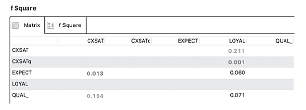
11. From Figure 41, the quadratic term CXSATq has a f² effect size of 0.001, which is smaller than the lower limit of 0.02 as proposed by Cohen (1988). The low f² effect size, combined with the non-significance of the quadratic effect, clearly suggests that customer satisfaction and loyalty have a linear relationship in our dataset.

Source: Ken Kwong-Kay Wong (2019), Mastering Partial Least Squares Structural Equation Modeling (Pls-Sem) with Smartpls in 38 Hours, iUniverse.