Chapter 4: Evaluating PLS-SEM Results in SmartPLS

1. The Colorful PLS-SEM Estimations Diagram

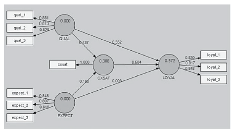
SmartPLS presents path modeling estimations not only in the Modeling Window but also in a text-based report³¹ which is accessible via the “Report” menu. In the PLS-SEM diagram, there are two types of numbers:

1. Numbers in the circle: These show how much the variance of the latent variable is being explained by the other latent variables.
2. Numbers on the arrow: These are called the path coefficients. They explain how strong the effect of one variable is on another variable. The weight of different path coefficients enables us to rank their relative statistical importance.³²

The PLS path modeling estimation for our restaurant example is shown in Figure 15.

Figure 15: PLS-SEM Results

Among all estimation results, the 3 key information that SmartPLS can inform you about the model are:

1. Outer loadings (in reflective measurement model) or outer weights (in formative measurement model)
2. Path coefficients for the structural model relationship
3. R² values of the latent endogenous variables

We will first explore these estimations results for model with reflective measurement scale in this Chapter 4, and then those with formative measurement scale in Chapter 5.

2. Initial Assessment Checklist

2.1. Model with Reflective Measurement

For an initial assessment of PLS-SEM, some basic elements should be covered in your research report. If a reflective measurement scale is used, as in our restaurant example, the following topics have to be discussed:

• Multicollineaiity Assessment
• Model’s f Effect Size
• Predictive Relevance: The Stone-Geisser’s (Q²) Values
• T otal Effect V alue
• Note: Indicator reliability, internal consistency reliability, and discriminant validity are only applicable to model having a reflective measurement scale.

2.2. Model with Formative Measurement

On the other hand, if the model uses a formative measurement scale, the following should be reported instead:

• Explanation of target endogenous variable variance
• Inner model path coefficient sizes and significance
• Outer model weight and significance
• Convergent validity
• Collinearity among indicators
• Checking Structural Path Significance in Bootstrapping
• Multicollinearity Assessment
• Model’s f² Effect Size
• Predictive Relevance: The Stone-Geisser’s (Q²) Values
• Total Effect Value

We will discuss model that utilizes formative measurement scale in greater details in the next chapter.

3. Evaluating PLS-SEM Model with Reflective Measurement

By looking at the PLS-SEM estimation diagram in Figure 15, we can make the following preliminary observations:

3.1. Explanation of Target Endogenous Variable Variance

• The coefficient of determination, R², is 0.572 for the LOYAL endogenous latent variable. This means that the three latent variables (QUAL, EXPECT, and CXSAT) moderately³⁴ explain 57.2% of the variance in LOYAL.
• QUAL and EXPECT together explain 30.8% of the variance of CXSAT.³⁵ Inner Model Path Coefficient Sizes and Significance
• The inner model suggests that CXSAT has the strongest effect on LOYAL (0.504), followed by QUAL (0.352) and EXPECT (0.003).
• The hypothesized path relationship between QUAL and LOYAL is statistically significant.
• The hypothesized path relationship between CXSAT and LOYAL is statistically significant.
• However, the hypothesized path relationship between EXPECT and LOYAL is not statistically significant³⁶. This is because its standardized path coefficient (0.003) is lower than 0.1. Thus, we can conclude that: CXSAT and QUAL are both moderately strong predictors of LOYAL, but EXPECT does not predict LOYAL directly.

3.2. Outer Model Loadings and Significance

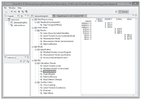
To view the correlations between the latent variable and the indicators in its outer model, go to “Report” in the menu and choose “Default Report”. Since we have a reflective model in this restaurant example, we look at the numbers as shown in the “Outer Loadings”— window (PLS-» Calculation Results -» Outer Loadings). We can press the “Toggle Zero Values” icon to remove the extra zeros in the table for easier viewing of the path coefficients (see Figure 16).

Figure 16: Path Coefficient Estimation in the Outer Model

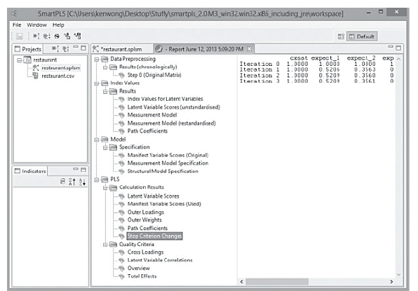
In SmartPLS, the software will stop the estimation when (i) the stop criterion of the algorithm was reached, or (ii) the maximum number of iterations has reached, whichever comes first. Since we intend to obtain a stable estimation, we want the algorithm to converge before reaching the maximum number of iterations. To see if that is the case, go to “Stop Criterion Changes” (see Figure 17) to determine how many iterations have been carried out. In this restaurant example, the algorithm converged only after 4 iterations (instead of reaching 300), so our estimation is good.

3. Indicator Reliability

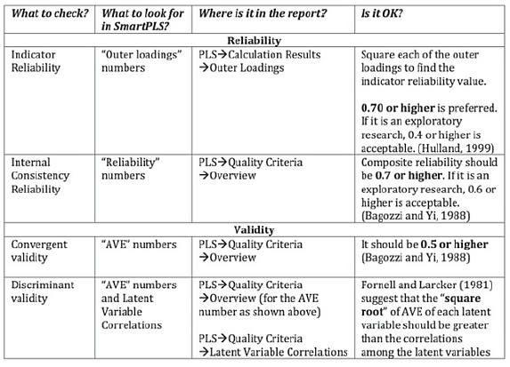
Just like all other marketing research, it is essential to establish the reliability and validity of the latent variables to complete the examination of the measurement model. The following table shows the various reliability and validity items that we must check and report when conducting a PLS-SEM (see Figure 18).

Figure 18: Checking Reliability and Validity

To report these reliability and validity figures, tables are often used for reporting purpose (see Figure 19).

Figure 19: Results Summary for Reflective Outer Models

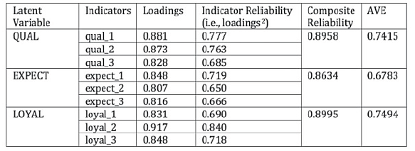
The first one to check is “Indicator Reliability” (see Figure 19). It can be seen that all of the indicators have individual indicator reliability values that are much larger than the minimum acceptable level of 0.4 and close to the preferred level of 0.7.

4. Internal Consistency Reliability

Traditionally, “Cronbach’s alpha” is used to measure internal consistency reliability in social science research but it tends to provide a conservative measurement in PLS-SEM. Prior literature has suggested the use of “Composite Reliability” as a replacement (Bagozzi and Yi, 1988; Hair et al., 2012). From Figure 19, such values are shown to be larger than 0.6, so high levels of internal consistency reliability have been demonstrated among all three reflective latent variables.

That said, the modern view of PLS suggests that instead of using Cronbach’s alpha and composite reliability, one should consider using “rho_A” coefficient to check the reliability of PLS construct scores, as defined in Dijkstra and Henseler (2015a). In SmartPLS v3, the “rho_A” value can be found in the Results Report (Quality Criteria -? Construct Reliability and Validity) once the PLS or PLSc Algorithm is performed. Generally speaking, a “rho_A” value of 0.7 or larger is preferred to demonstrate composite reliability. Meanwhile, a “rho_A” value above 1 is abnormal and should not occur in the model.

6. Convergent Validity

To check convergent validity, each latent variable’s Average Variance Extracted (AVE) is evaluated. Again from Figure 19, it is found that all of the AVE values are greater than the acceptable threshold of 0.5, so convergent validity is confirmed.

7. Discriminant Validity

There are two ways to check discriminant validity: the Fomell-Larcker Criterion and HTMT. The classical approach is proposed by Fornell and Larcker (1981) who suggest that the square root of AVE in each latent variable can be used to establish discriminant validity, if this value is larger than other correlation values among the latent variables. To do this, a table is created in which the square root of AVE is manually calculated and written in bold on the diagonal of the table. The correlations between the latent variables are copied from the “Latent Variable Correlation” section of the default report and are placed in the lower left triangle of the table (see Figure 20).

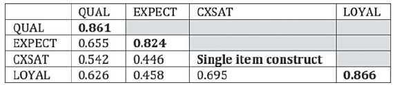
For example, the latent variable EXPECT’s AVE is found to be 0.6783 (from Figure 19) hence its square root becomes 0.824 (see Figure 20). This number is larger than the correlation values in the column of EXPECT (0.446 and 0.458) and also larger than those in the row of EXPECT (0.655). Similar observation is also made for the latent variables QUAL, CXSAT and LOYAL. The result indicates that discriminant validity is well established.

The modern approach to check discriminant validity is to use Heterotrait-monotrait ratio of correlations (HTMT) that is proposed by Henseler, Ringle and Sarstedt (2015). This procedure can be performed in SmartPLS v3 easily and the step-by-step procedure is shown in Chapter 12.

8. Checking Structural Path Significance in Bootstrapping

SmartPLS can generate T-statistics for significance testing of both the inner and outer model, using a procedure called bootstrapping. In this procedure, a large number of subsamples (e.g., 5000) are taken from the original sample with replacement to give bootstrap standard errors, which in turn gives approximate T-values for significance testing of the structural path. The Bootstrap result approximates the normality of data.

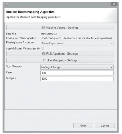
To do this, go to the “Calculate” menu and select “Bootstrapping”. In SmartPLS, sample size is known as Cases within the Bootstrapping context, whereas the number of bootstrap subsamples is known as Samples. Since there are 400 valid observations⁴² in our restaurant data set, the number of “Cases” (not “Samples”) in the setting should be increased to 400 as shown in Figure 21. The other parameters remain unchanged:

1. Sign Change: No Sign Changes
2. Cases: 400
3. Samples: 5000

It worth noting that if the bootstrapping result turns out to be insignificant using the “No Sign Changes” option, but opposite result is achieved using the “Individual Sign Changes” option, you should subsequently re-run the procedure using the middle “Construct Level Changes” option and use that result instead. This is because this option is known to be a good compromise between the two extreme sign change settings.

Figure 21: Bootstrapping Algorithm

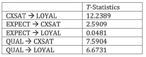
Once the bootstrapping procedure is completed, go to the “Path Coefficients (Mean, STDEV, T-Values) window located within the Bootstrapping section of the Default Report. Check the numbers in the ‘T-Statistics” column to see if the path coefficients of the inner model are significant or not. Using a two-tailed t-test with a significance level of 5%, the path coefficient will be significant if the T-statistics⁴³ is larger than 1.96. In our restaurant example, it can be seen that only the “EXPECT – LOYAL” linkage (0.0481) is not significant. This confirms our earlier findings when looking at the PLS-SEM results visually (see Figure 15). All other path coefficients in the inner model are statistically significant (see Figure 22 and 23)

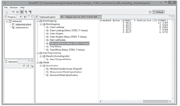
Figure 23: T-Statistics of Path Coefficients (Inner Model)

After reviewing the path coefficient for the inner model, we can explore the outer model by checking the T- statistic in the “Outer Loadings (Means, STDEV, T-Values)” window. As presented in Figure 24, all of the T- Statistics are larger than 1.96 so we can say that the outer model loadings are highly significant. All of these results complete a basic analysis of PLS-SEM in our restaurant example.

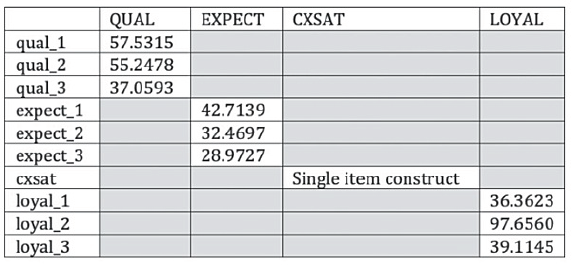
Figure 24: T-Statistics of Outer Loadings

9. Multicollinearity Assessment

The depth of the PLS-SEM analysis depends on the scope of the research project, the complexity of the model, and common presentation in prior literature. For example, a detailed PLS-SEM analysis would often include a multicollinearity assessment. That is, each set of exogenous latent variables in the inner model⁴⁴ is checked for potential collinearity problem to see if any variables should be eliminated, merged into one, or simply have a higher- order latent variable developed.

To assess collinearity issues of the inner model, the latent variable scores (PLS -> Calculation Results Latent Variable Scores) can be used as input for multiple regression in IBM SPSS Statistics to get the tolerance or Variance Inflation Factor (VIF) values, as SmartPLS does not provide these numbers. First, make sure the data set is in .csv file format. Then, import the data into SPSS and go to Analyze Regression -> Linear. In the linear regression module of SPSS, the exogenous latent variables (the predictors) are configured as independent variables, whereas another latent variable (which does not act as a predictor) is configured as the dependent variable. VIF is calculated as “1/Tolerance”. As a rule of thumb, we need to have a VIF of 5 or lower (i.e., Tolerance level of 0.2 or higher) to avoid the collinearity problem (Hair et al., 2011).

10. Model’s —Effect Size

In addition to checking collinearity, there can be a detailed discussion of the model’s f² effect size which shows how much an exogenous latent variable contributes to an endogenous latent variable’s R² value. In simple terms, effect size assesses the magnitude or strength of relationship between the latent variables. Such discussion can be important because effect size helps researchers to assess the overall contribution of a research study. Chin, Marcolin, and Newsted (1996) have clearly pointed out that researcher should not only indicate whether the relationship between variables is significant or not, but also report the effect size between these variables.

11. Predictive Relevance: The Stone-Geisser’s (Q2) Values

Meanwhile, predictive relevance is another aspect that can be explored for the inner model. The Stone-Geisser’s (Q²) values⁴⁶ (i.e., cross-validated redundancy measures) can be obtained by the Bindfolding procedure in SmartPLS (Calculate -> Bindfolding). In the Bindfolding setting window, an omission distance (OD) of 5 to 10 is suggested for most research (Hair et al., 2012). The q² effect size for the Q² values can also be computed and discussed.

12. Total Effect Value

If a mediating latent variable exists in the model, one can also discuss the Total Effect of a particular exogenous latent variable on the endogenous latent variable. Total Effect value can be found in the default report (PLS Quality Criteria -> Total Effects). The significance of Total Effect can be tested using the T-Statistics in the Bootstrapping procedure (Bootstrapping Total Effects (Mean, STDEV, T-Values)). Also, unobserved heterogeneity may have to be assessed when there is little information about the underlying data, as it may affect the validity of PLS-SEM estimation. See Chapter 8 for a detailed discussion on the issue of heterogeneity.

13. Managerial Implications – Restaurant Example

The purpose of this example is to demonstrate how a restaurant manager can improve his/her business by understanding the relationships among customer expectation (EXPECT), perceived quality (QUAL), customer satisfaction (SAT) and customer loyalty (LOYAL). Through a survey of the restaurant patrons and the subsequent structural equation modeling in SmartPLS, the important factors that lead to customer loyalty are identified.

In this research, customers are found to care about food taste, table service, and bill accuracy. With loadings of 0.881, 0.873 and 0.828 respectively, they are good indicators of perceived quality (QUAL). Restaurant management should not overlook these basic elements of day-to-day operation because perceived quality has been shown to significantly influence customers’ satisfaction level, their intention to come back, and whether or not they would recommend this restaurant to others.

Meanwhile, it is also revealed that menu selection, atmospheric elements and good-looking staff are important indicators of customer expectation (EXPECT), with loadings of 0.848, 0.807, and 0.816 respectively. Although fulfilling these customer expectations can keep them satisfied, improvement in these areas does not significantly impact customer loyalty due to its weak effect (0.03) in the linkage. As a result, management should only allocate resources to improve these areas after food taste, table service and bill accuracy have been looked after.

The analysis of inner model shows that perceived quality (QUAL) and customer expectation (EXPECT) together can only explain 30.8% of the variance in customer satisfaction (CXSAT). It is an important finding because it suggests that there are other factors that restaurant managers should consider when exploring customer satisfaction in future research.

Source: Ken Kwong-Kay Wong (2019), Mastering Partial Least Squares Structural Equation Modeling (Pls-Sem) with Smartpls in 38 Hours, iUniverse.