1. Case Study: Customer Survey in a Photocopier Manufacturer (B2B)
Since PLS-SEM is a relatively new approach to modeling, researchers who are not familiar with it may find the analytical and reporting aspects challenging, especially in the areas of higher-order constructs modeling, mediation analysis, and categorical moderation analysis. Chapter 9, 10 and 11 are written to help researchers master these skill sets by demonstrating the mentioned analyses through a fictitious B2B research example in the photocopier industry. PLS-SEM model estimation was performed in SmartPLS 2.0M3 software (Ringle, C. M., Wende, S., & Will, A., 2005), whereas data preparation will be performed in Microsoft Excel and IBM SPSS.
2. Conceptual Framework and Research Hypotheses
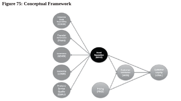
In this research example, a researcher named Susan is the marketing vice president of a photocopier manufacturer. The company’s business customers include organizations in both non-profit and for-profit sectors. Susan is interested in learning more about the driving forces behind customer loyalty, particularly factors such as brand reputation, pricing, and customer satisfaction. Susan has previously attended an EMBA course on brand reputation, and she recalled the 5 underlying indicators that contribute to a company’s brand reputation; they are corporate social responsibility, financial performance, governance, leadership, and product/service quality. Susan is interested in carrying out a structural equation modeling exercise because her goal is to understand the relationships among these factors. Based on this information, Susan developed the conceptual framework for her research project (see Figure 75).
3. Questionnaire Design and Data Collection
A questionnaire is designed around each latent construct of interest. Susan’s business customers are asked to provide feedback in major areas that reflect the latent constructs in the model. Using a measurement scale from 0 to 10 (totally disagree to fully agree), business customers are asked to evaluate each statement (i.e., the indicator variable) such as “This company offers good after-sales service.” in the questionnaire. Since brand reputation is a higher-order construct, it is evaluated by asking questions surrounding the 5 underlying factors. The statements to be evaluated are:
Quality (QUALI)
[This company] offers reliable, high-quality photocopier.
[This company] offers good after-sales service.
Corporate Social Responsibility (COSOR)
[This company] sponsors community events and programs.
[This company] maintains production processes that minimize the impact to the environment.
Financial Performance (FINAN)
[This company] is a high-performance company, it delivers strong financial results.
[This company] delivers above-market-average share price performance.
[This company] has a comfortable cash position.
Governance (GOVER)
[This company] behaves ethically and is open and transparent in its business dealings.
[This company] has good internal control.
[This company] maintains full compliance in its financial disclosures and reports.
Leadership (LEADR)
[This company] has a strong, visible leader.
[This company] is managed effectively.
The senior management is well known for its good relationship with its employees.
Pricing (PRICE)
The price is reasonable.
The total cost of ownership reasonable.
Customer Loyalty (LOYAL)
I would recommend [this company] to other business partners.
If I had to select again, I would choose [this company] as my photocopier supplier.
I will remain a customer of [this company] in the future.
Customer Satisfaction (SATIS)
Overall, I am satisfied with the product and service provided by [this company].
A total of 200 questionnaires are received from Susan’s business customers; 106 of them are non-profit organizations (including government agencies) whereas the rest are for-profit companies. Luckily, the collected questionnaires contain no missing data.
4. Hypotheses Development
Once the conceptual framework is finalized, the next step is hypotheses development. The first hypothesis is developed to explore the relationship between brand reputation and loyalty:
Hi’- Brand reputation (REPUT) significantly influences customer loyalty (LOYAL)
The second hypothesis is developed to examine the relationship between brand reputation and customer satisfaction:
H2: Brand reputation (REPUT) significantly influences customer satisfaction (SATIS)
The third and fourth hypotheses are created to explore the relationship between pricing and customer loyalty, and those between pricing and customer satisfaction, respectively:
H3: Pricing (PRICE) significantly influences customer loyalty (LOYAL)
H4: Pricing (PRICE) significantly influences customer satisfaction (SATIS)
The fifth hypothesis is created to test the linkage between customer satisfaction and customer loyalty:
H5: Customer satisfaction (SATIS) significantly influences customer loyalty (LOYAL)
Customer satisfaction is an endogenous variable in the model. Other latent constructs such as brand reputation and pricing are hypothesized to influence customer satisfaction, which in turn affects customer loyalty. The potential mediating effect of customer satisfaction on other constructs are of interest in Susan’s research and hence the sixth and seventh hypothesis are developed as the followings:
H6: Customer satisfaction (SATIS) significantly mediates the relationship between brand reputation (REPUT) and customer loyalty (LOYAL)
H7: Customer satisfaction (SATIS) significantly mediates the relationship between pricing (PRICE) and customer loyalty (LOYAL)
Susan is also interested in understanding if her findings in this PLS-SEM research can be applied to both nonprofit and for-profit organizations. To confirm such insights, the last hypothesis of this research is developed to test the categorical moderating effect of business type (i.e., non-profit vs. for-profit) in the model:
H8: There is significant categorical moderating effect of business type on the relationship among model constructs.
We will explore mediation analysis later in Chapter 10, followed by categorical moderation analysis in Chapter 11.
5. PLS-SEM Design Considerations Sample size
In Susan’s research project, there are 200 participants (N=106 non-profit organizations; N=94 for-profit organizations). This sample size satisfies both the “10 times rule”65 (Thompson, Barclay, & Higgins, 1995) and the guidelines66 as suggested by Hair, Hult, Ringle, & Sarstedt (2013).
6. Multiple-item vs. Single-item Indicators
This research originally includes a total of 19 indicator variables. Since the sample size is larger than 50, the indicating variables are designed to make use of multiple-item instead of single-item to measure the latent construct (Diamantopoulos, Sarstedt, Fuchs, Kaiser, & Wilczynski, 2012). Other than customer satisfaction (SATIS) which is a single-item construct, all others are each measured by 2 to 3 indicators (i.e., questionnaire questions).
7. Formative vs. Reflective Hierarchical Components Model
According to Lohmoller (1989), PLS-SEM can be designed as a hierarchical components model (HCM)67 that includes the observable lower-order components (LOCs) and unobservable higher-order components (HOCs) to reduce model complexity and make it more theoretical parsimony.
In Susan’s photocopier research, it is designed as a reflective-reflective hierarchical component model (rr- HCM)68. Specifically, the HOC brand reputation holds a reflective relationship with its LOCs (quality, corporate social responsibility, financial performance, governance, and leadership) that are measured by reflective indicators that hang well together. This model design is in line with prior research regarding reputation for company (Hair et al., 2013, p235).
8. Data Preparation for SmartPLS
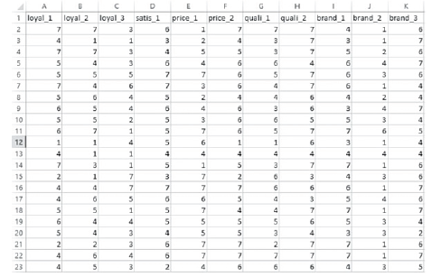
Prior to running PLS model estimation in SmartPLS, Susan has to manually type the questionnaire data into Microsoft Excel with the names of those indicators (e.g., loyal_1, loyal_2, loyal_3) being placed in the first row of an Excel spreadsheet. Each row represents an individual questionnaire response, with number from 0 to 10. Since there are 200 responses, there should be 201 rows in the spreadsheet (see Figure 76). The file has to be saved in the specific “CSV (Comma Delimited)” format in Excel69 because SmartPLS cannot import .xls or .xlsx files directly. Figure 76: Data Entry in Microsoft Excel
9. Data Analysis and Results PLS Path Model Estimation
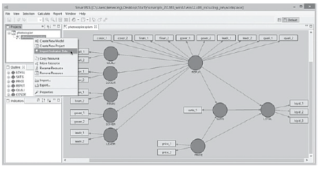
Susan designs the PLS model in SmartPLS based on the conceptual framework mentioned earlier. The HOC, brand reputation, is drawn using the “repeated indicators approach”70. Once the model is drawn, the indicator data can be imported into the SmartPLS software71 (see Figure 77).
The PLS-SEM algorithm is run72 and successfully converged73 within the guideline suggested by Hair et al., (2013). Before Susan can properly assess the path coefficients in the structural model, she must first examine the indicator reliability, internal consistency reliability, discriminant validity, and convergent validity of the reflective measurement model to ensure they are satisfactory (Wong, 2013).
10. Indicator Reliability
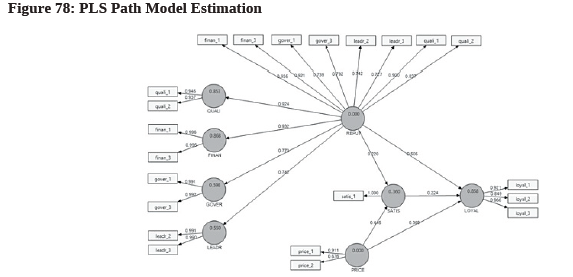
Since reliability is a condition for validity, indicator reliability is first checked to ensure the associated indicators have much in common that is captured by the latent construct. After examining the outer loadings for all latent variables74, the 2 indicators that form COSOR are removed because their outer loadings are smaller than the 0.4 threshold level (Hair et al, 2013). Meanwhile, 3 indicators (Finan_2, Gover_2, and Leadr_1) are found to have loadings between 0.4 to 0.7. A loading relevance test75 is therefore performed for these 3 indicators to see if they should be retained in the model. As the elimination of these 3 indicators would result in an increase of Average Variance Extracted (AVE) and composite reliability of their respective latent construct, they are removed from the PLS model. The remaining indicators are retained because their outer loadings are all 0.7 or higher76. The PLS algorithm is re-run. The resulting path model estimation is presented in Figure 78 and the outer loadings of various constructs are shown in Figure 79:
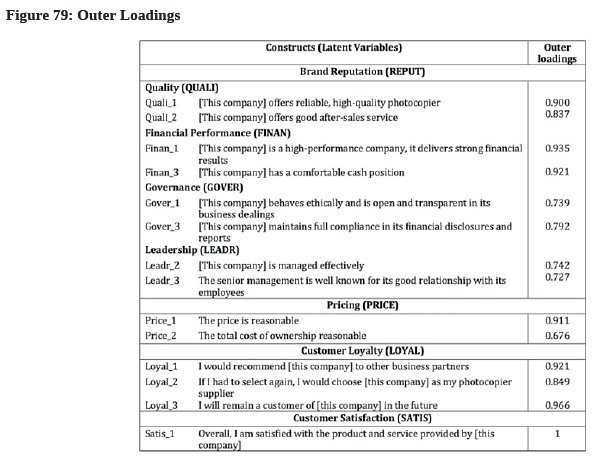
11. Internal Consistency Reliability
In this PLS-SEM example, composite reliability rather than Cronbach’s alpha77 is used to evaluate the measurement model’s internal consistency reliability.78 This is because it takes into consideration of the different outer loadings of the indicators (Werts, Linn, & Joreskog, 1974). In Susan’s research, the composite reliability79 for the constructs REPUT, PRICE and LOYAL are shown to be 0.9454, 0.7791, and 0.9378 respectively, indicating high levels of internal consistency reliability80 (Nunnally & Bernstein, 1994). Please note that the value of SATIS is 1.00 but it does not imply perfection in composite reliability because it is a single-item variable.
12. Convergent Validity
Convergent validity refers to the model’s ability to explain the indicator’s variance. The AVE can provide evidence81 for convergent validity (Fornell and Larcker, 1981). The AVE for the latent construct LOYAL, PRICE, and REPUT are 0.8343, 0.6432, and 0.6859 respectively, well above the required minimum level of 0.50 (Bagozzi and Yi, 1988). Therefore, the measures of the three reflective constructs can be said to have high levels of convergent validity.
13. Discriminant Validity
As discussed previously in the book, the Fornell-Larcker criterion (1981) is a traditional and common approach to assess discriminant validity82 although it gives conservative results as compared to the modern approach of using HTMT (see Chapter 12 if HTMT is chosen to check discriminant validity).
If the Fornell-Larcker criterion is used, the AVE should be checked. That is, in order to establish the discriminant validity83, the square root of average variance extracted (AVE) of each latent variable should be larger than the latent variable correlations (LVC). Figure 80 clearly shows that discriminant validity is met for this research because the square root of AVE for REPUT, PRICE, SATIS and LOYAL are much larger than the corresponding LVC84.
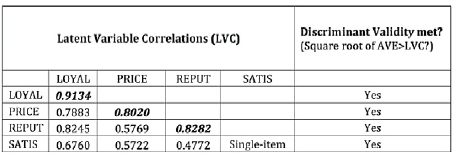
Note: The square root of AVE values is shown on the diagonal and printed in italics; non-diagonal elements are the latent variable correlations (LVC).
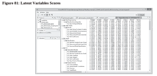
14. Collinearity Assessment
In addition to checking the measurement model, the structural model has to be properly evaluated before drawing any conclusion. Collinearity is a potential issue in the structural model and that variance inflation factor (VIF) value of 5 or above typically indicates such problem (Hair et al., 2011). Since SmartPLS does not generate the VIF value, another piece of statistical software such as IBM SPSS has to be utilized. This procedure involves a few easy steps. First, generate the latent variables scores85 in SmartPLS (see Figure 81).
Then, copy the data into Microsoft Excel, save it in “CSV (Comma Delimited)” format and then open it in IBM SPSS (see Figure 82).
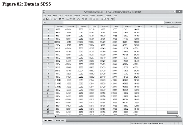
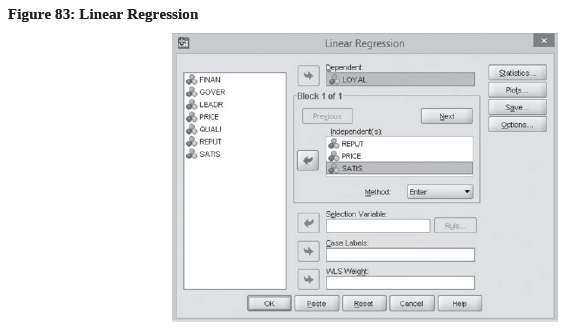
In Susan’s PLS model, both LOYAL and SATIS act as dependent variables because they have arrows (paths) pointing toward them. So, we need to run two different sets of linear regression to obtain their corresponding VIF values.
For the first run of linear regression86, LOYAL is the dependent variable whereas REPUT, PRICE, and SATIS serve as “Independent” variables (see Figure 83).
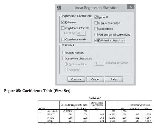
In the Linear Regression window, click the “Statistics…” button and then put a check mark next to “Collinearity diagnostics” (see Figure 84) to obtain the VIF value (see Figure 85).
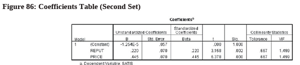
For the second set of linear regression, configure SATIS as dependent variable and REPUT and PRICE as independent variables. The VIF values are shown in Figure 86.
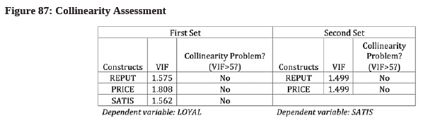
The collinearity assessment results are summarized in Figure 87. It can be seen that all VIF values are lower than 5, suggesting that there is no indicative of collinearity between each set of predictor variables.
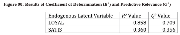
15. Coefficient of Determination (R2)
A major part of structural model evaluation is the assessment of coefficient of determination (R2). In Susan’s research, LOYAL is the main construct of interest. From the PLS Path model estimation diagram (see Figure 78), the overall R2 is found to be a strong87 one, suggesting that the three constructs REPUT, PRICE, and SATIS can jointly explain 85.8% of the variance of the endogenous construct LOYAL88. The same model estimation also reveals the R2 for other latent construct; REPUT and PRICE are found to jointly explain 36.0% of SATIS’s variances in this PLS-SEM model.
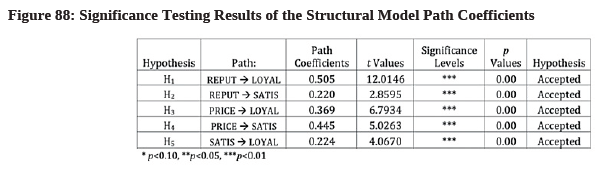
16. Path Coefficient
In SmartPLS, the relationships between constructs can be determined by examining their path coefficients and related t statistics via the bootstrapping procedure89. From Figure 88, it can be seen that all of the structural model relationships are significant90, confirming our various hypotheses about the construct relationships. The PLS structural model results enable us to conclude that REPUT has the strongest effect on LOYAL (0.505), followed by PRICE (0.369) and SATIS (0.224).
The PLS model estimation (see Figure 78) also reveals that the high-order construct, REPUT, has strong relationships91 with its low-order constructs, QUALI (0.924), FINAN (0.932), GOVER (0.773) and LEADR (0.742).
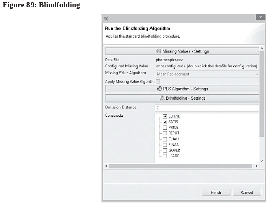
16. Predictive Relevance (Q2)
An assessment of Stone-Geisser’s predictive relevance (Q2) is important because it checks if the data points of indicators in the reflective measurement model of the endogenous construct can be predicted accurately. This can be achieved by making use of the blindfolding procedure92 in SmartPLS (see Figure 89).
The following table summarizes the results93. It is observed that the proposed model has good predictive relevance94 for all of the endogenous variables (see Figure 90).
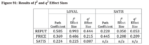
17. The f2 and q2 Effect Sizes
The final step in structural model evaluation is to assess the effect of a specific exogenous construct on the endogenous construct if it is deleted from the model. This can be achieved by examining the f2 and q2 effect sizes, which can be derived from R2 and Q2 respectively95. Following Cohan’s (1988) guideline96, it can be said that in general, the exogenous variables have medium to large f2 and q2 effect sizes on the endogenous variables (see Figure 91).
Source: Ken Kwong-Kay Wong (2019), Mastering Partial Least Squares Structural Equation Modeling (Pls-Sem) with Smartpls in 38 Hours, iUniverse.
28 Sep 2021
28 Sep 2021
28 Sep 2021
28 Sep 2021
28 Sep 2021
28 Sep 2021