1. Something is Hiding in the Dataset
In exploratory research, marketing researchers may have little knowledge about the nature of the underlying data. They need to consider the potential problem of heterogeneous data structures in PLS-SEM modeling because the data do not necessarily come from a homogeneous population (see Figure 42).
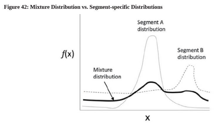
If heterogeneity is established, researchers may need to estimate two or more separate models to avoid drawing an incorrect conclusion about the model relationships (Sarstedt, Schwaiger, & Ringle, 2009). There are two kinds of heterogeneity: observed and unobserved ones. Observed heterogeneity often happens between two or more groups due to the presence of a categorical moderator variable, such as demographic differences (e.g., age, gender, or nationality). On the other hand, unobserved heterogeneity may occur without driven by obvious, observable group characteristics. Researchers need to treat unobserved heterogeneity because it biases parameter estimates, threatens different types of validity50 due to Type I and Type II errors, and leads to invalid conclusions51 (Jedidi et al., 1997).
2. Establishing Measurement Invariance (MICOM)
Before running any multigroup analysis, researchers need to first establish measurement invariance52 in PLS-SEM in order to eliminate measurement error and protect the validity of the outcomes. This can be achieved by using the “Measurement Invariance of the Composite Models” (MICOM) procedure as proposed by Henseler, Ringle, and Sarstedt (2016). If measurement invariance is not established prior to performing multi-group analysis, the conclusion can be questionable because the model may suffer from low power of statistical tests and low precision of estimators (Hult et al., 2008).
The MICOM procedure consists of 3 steps that should be completed in sequence. The first step is to test “Configural invariance”, the second step is to test “Compositional invariance”. The third step is to test “composite means and variances”. Both the configural invariance and compositional invariance have to be established prior to running any multi-group analysis. If either one is not established, researchers should analyze the groups separately and not performing any multi-group analysis. Once these two invariances are both established, the equality of composite means and variances can be checked. If they are equal, full measurement invariance is established. This means that multigroup analysis can be performed and pooling of data is possible. Otherwise, partial measurement invariance is established, meaning multigroup analysis can still be performed but pooling of data is not possible.
3. Modeling Observed Heterogeneous Data
Different kinds of techniques have been proposed to handle a priori groupings in multi-group analysis53 (Keil et al, 2000; Sarstedt and Mooi, 2014; Henseler et al., 2009; Chin and Dibbern, 2010). To compare two groups of data in PLS-SEM specifically54, the non-parametric “Permutation test” is suggested due to its advantageous statistical properties, such as having no data distributional assumptions and being able to perform well across a broad range of conditions (Ernst, 2004; Good, 2000).
4. Permutation Test Procedures
- Let us use the “cafe100” dataset again for illustration. In this example, the cafe patrons can be categorized into 2 groups: students (code: 1) and non-students (code: 2).
- In SmartPLS, under the “Project Explorer” tab in the upper left-hand side of the window, double click the “cafe100 [100 records]” data file which has a green icon.
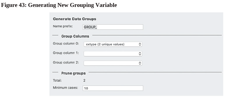
- At the top of the window, there is a button called “Generate Data Groups”. Click it to create a new grouping variable.
- In the “Generate Data Groups” window, click the “Group column 0:” pull-down menu to select “cxtype (2 unique values)” (see Figure 43):

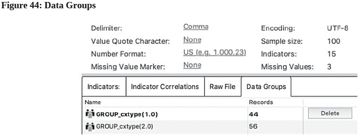
- Press OK. You should be able to see the customer distribution information as in Figure 44:
- Go back to the colorful “Cafe100.splsm” model tab. In the “Calculate” menu, select “Permutation”. Under the “Setup” tab, click the “Group A” pull-down menu to select “GROUP_cxtype(1.0)”. Similarly, click the “Group B” pull-down menu to select “GROUP_cxtype(2.0)” (see Figure 45):
- Start calculation using the following parameters:
- Permutations: 1000
- Test Type: Two Tailed
- Significance Level: 0.05
- Do Parallel Processing: Checked [ticked]
- To establish “Configural invariance” as in Step 1 of the MICOM procedure, we need to ensure that (i) the PLS path models, (ii) data treatment, and (iii) algorithm settings of both groups are exactly the same. Since this is the case when we perform the permutation model estimation, we have established configural invariance.
- Next, we want to establish “Compositional invariance” as in Step 2 of the MICOM procedure. To do this, we examine the “Permutation p-Values” of the constructs. Select the MICOM hyperlink under the “Quality Criteria” heading at the bottom of the result page and look at the last column in the “Step 2” tab (see Figure 46).
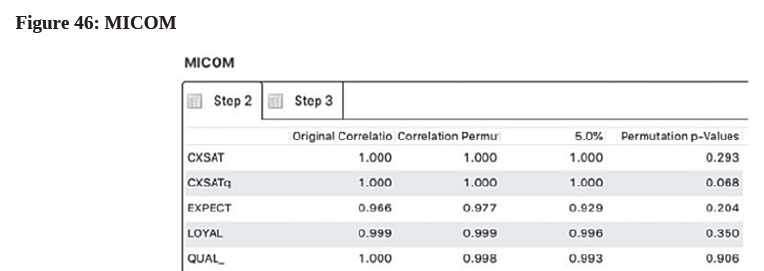
- Since all constructs have their “Permutation p-Values” larger than 0.05, we accept the null hypothesis that the original correlations of these constructs are not significantly different from 1. This gives us supporting evidence that compositional invariance has been established in the model.
- We can proceed to check whether we have achieved full measurement invariance or just partial measurement invariance by looking at the composite means and variances, as in Step 3 of MICOM. This information is presented in the “Step 3” tab (see Figure 47).
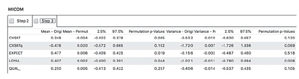
- The first few columns show information about the Mean, whereas the last 5 columns show information about the Variance. From Figure 47, it can be seen that not all of the mean’s “Permutation p-value” are larger than
- Similarly, in terms of variance, some constructs have their “Permutation p-value” smaller than 0.05, we, therefore, accept the alternative hypothesis that there are significant differences in the composite mean values and variances of latent variables across the two groups. In other words, we can only establish partial measurement invariance because not all the composite mean values and variances are equal.
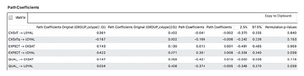
- The final step is to explore the path coefficients. Look at the “Final Results” heading and select the “Path Coefficients” hyperlink at the bottom of the result page. Compare the path coefficients of the groups (see first two columns in Figure 48) and also look at their “Permutation p-Values” in the last column.
- From Figure 48, it can be seen that the 2 key linkages, “EXPECT LOYAL” and “QUAL LOYAL”, both have a Permutation p-values of 0.039. This means that effect between EXPECT and LOYAL is significantly (p<0.05) different between cafe patrons who are students (p1=0.422) and those who are non-students (p2=0.071). Similarly, we can draw the conclusion that effect between QUAL and LOYAL is significantly (p<0.05) different between cafe patrons who are students (p1=0.034) and those who are non-students (p2=0.408).
- Reviewing the original survey questions and the above results can help the cafe manager to draw some managerial implications. We can argue that students care more about the Customer Expectation (EXPECT) than non-students, when it comes to affecting their loyalty intentions. This argument is logical, one of the indicators for the EXPECT construct, expect_4, is related to affordable daily special dishes. If the cafe owner would like to continue earning loyalty from the students, it is advisable for the cafe owner to keep the daily specials and not removing it from the menu.
- Similarly, the result shows that non-students put a heavier focus on the Perceived Quality (QUAL). This is not surprising as one of the indicators, qual_4, refers to how well the cafe can craft alcoholic drinks, something that only excites the more matured, non-student cafe patrons.
4. Modeling Unobserved Heterogeneous Data
When there are suspicious differences in structural path coefficients but the existing theory does not assume heterogeneity, the model may be affected by unobserved heterogeneity. Many tools have been proposed to identify and treat such heterogeneity in PLS-SEM–, but researchers have recommended the use of “latent class techniques”56 such as Finite Mixture Partial Least Squares (FIMIX-PLS) (Sarstedt, Becker, Ringle, & Schwaiger, 2011) and PLS Prediction-oriented Segmentation (PLS-POS) (Becker, Rai, Ringle, and Volckner, 2013). These two techniques are handy because FIMIX-PLS is an effective tool to reveal the number of segments hiding in the underlying data, whereas PLS-POS can then be used to explain the structure of latent segment and estimate segment-specific models.
When the PLS path models include formative measures, PLS-POS is preferred over other latent class techniques for checking unobserved heterogeneity in both structural and measurement models. This method manages heterogeneity by using a distance measure that facilitates the reassignment of observations with the objective of improving the prediction-oriented optimization criterion (Becker et al., 2013).
Once FIMIX-PLS and PLS-POS are performed, researchers can carry out ex-post analysis to identify explanatory variables and elaborate on the theory. By turning unobserved heterogeneity into observed heterogeneity in the dataset, researchers can then test and validate the segment-specific path models. As pointed out by Becker et al. (2013), a well-defined segment should be substantial, differentiable, plausible, and accessible. These are the important checkpoints when we go through the process of modeling unobserved heterogeneous data.
5. FIMIX-PLS Procedures
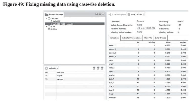
- The first step of FIMIX-PLS is to manage missing data in the dataset. If there are missing values, researchers should delete those observations that have missing values using the casewise deletion method, instead of replacing them with the mean value. To find out if there are any missing values in the dataset, click the green icon of the data file “cafe100 [100 records]” and then look at the “cafe100.txt” tab on the right-hand side of the screen. Go to the “Indicators:” tab and look at the “Missing” column. From the following Figure 49, we can see that there is a total of 3 incomplete observations in our “cafe100” dataset.
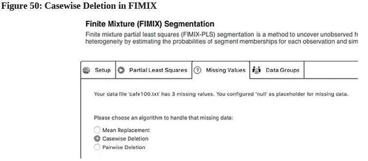
- There are some missing values in the indicators expect_1, expect_4, and qual_1. To address this problem, first click the colorful “Cafe100.splsm” tab. Go to the “Calculate” menu and select “Finite Mixture (FIMIX) Segmentation”. Then, view the “Missing Values” tab and select “Casewise Deletion” (see Figure 50). Note that if there are no missing values in the dataset, this “Missing Values” tab will not be shown at all in FIMIX.
- Since we are exploring unobserved heterogeneous data, we do not know precisely how many relevant segments (or groups) there are in the dataset a priori. Although we can use a common approach to determine the potential number of segments such as dividing the number of observations by the minimum sample size57, we can also make an educated guess by considering the model background, the data distributional characteristics, and the variables’ psychometric properties. As we have a small dataset with only 97 observations after casewise deletion, we tentatively suggest the potential presence of 4 customer segments to begin the FIMIX-PLS procedure and let the results confirm this number.
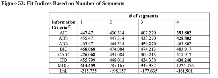
- Create a table like the following one to show the index fit:
(Note: For the fit measure in each information criterion, the optimal solution is the number of segments with the lowest value. The only exception is LnL (LogLikeihood) where the bigger the value, the better it is0
- Go back to the “Setup” tab to perform FIMIX-PLS calculation using the following parameters:
- Number of Segments: 1 [Yes, select 1 and not 2 here to create our initial estimation]
- Maximum number of iterations: 5000
- Stop Criterion: 5 (-Jl.OE-5) [If you see a red icon there, just click the arrow up and then down]
- Number of Repetitions: 10
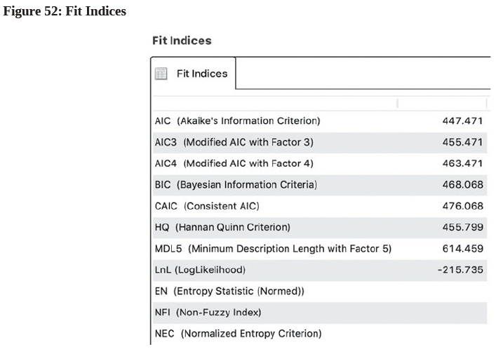
- On the FIMIX result page, first check the fit indices by going to the “Quality Criterion” heading and clicking the “Fit indices” hyperlink for a model with only one segment. Copy the data (see Figure 52) and paste them into the table created in step 4.
- Since we made an educated guess about having 4 segments in the dataset, re-run the FIMIX-PLS calculation using the following parameters in the “Setup” tab:
- Number of Segments: 4
- Maximum number of iterations: 5000
- Stop Criterion: 5 (->1.0E-5) [If you see a red icon there, just click the arrow up and then down]
- Number of Repetitions: 10
- Check the fit indices once again by going to the “Quality Criterion” heading and selecting “Fit indices” for a model with two segments. Copy the data and paste them into the table. Following this logic, if you have 5 potential segments in your dataset, for example, you have to create a table with 5 columns for the segments and then run the FIMIX-PLS procedure 5 times (i.e., first time with 1 segment, second time with 2 segments, third time with 3 segments.. .etc.) using different number of segments to find out their corresponding Fit Indices.
- In each row, we bold the optimal fit index value. For example, in the AIC row, we bold the value 393.802 as it is the lowest value, whereas in the LnL row, we bold the-161.901 as it is the highest value. From Table 4, we can see that the 1-segment model has 3 optimal solutions (i.e., only BIC, CAIC, and MDL5 are in bold), the 2- segment model has no optimal solution, the 3-segment solution has just 1 optimal solution (i.e., AIC4 is in bold), whereas the 4-segment model has the most number of optimal solutions (i.e., AIC, AIC3, HQ and LnL are in bold). This leads us to believe that the dataset has 4 underlying segments technically speaking.
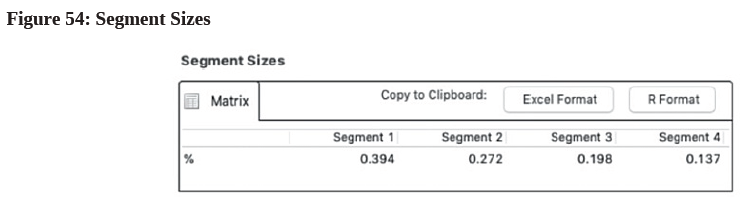
- As discussed earlier, the segments should be substantial in size to represent a “real” segment. Researcher needs to eliminate the small segments58 that are irrelevant for theory or practice. We can also look at their sample sizes by going to the Result report and clicking the “Segment Sizes” hyperlink under the “Final Results” heading. From Figure 54, it can be seen that Segment 1 is 39.4% of the data, Segment 2 is 27.2% of the data, Segment 3 is 19.8% of the data, whereas Segment 4 is the smallest one that makes up 13.7% of the data. These segments are big enough in general for our modeling. In case the resulting segment(s) are tiny (e.g., 2%), marketing researcher should consider eliminating them from the investigation as they are not substantial.
- Using FIMIX-PLS, we conclude that there are 4 segments in our “cafe100” dataset.
- The next step is to better understand the data in each of these identified segments. The FIMIX-PLS technique that we have just performed is limited to uncovering unobserved heterogeneity in the structural model only, it cannot handle model with formative measures properly. Meanwhile, the other statistical procedure, PLS-POS, can reveal unobserved heterogeneity in both the measurement and structural models. As such, PLS-POS is highly recommended for exploring the identified segments further, such as calculating the average explained variance R2 and path coefficients. In other words, we should use FIMIX-PLS only to identify the number of segments presented in the dataset and then use PLS-POS to explore the remaining properties of the model.
6. PLS-POS Procedures
- Click the colorful “Cafe100.splsm” model tab. Go to the “Calculate” menu and select “Prediction-Orientation Segmentation (POS)”. In the “Setup” tab, start calculation use the following parameters:- Groups: 4 [based on our FIMIX-PLS result where it identified 4 segments]- Maximum Iterations: 1000 [Multiply our number of observations by 2 and compare that to the default value of 1000. Then, select the higher of the two]
– Search Depth: 100 [this should equal the number of observations, which is 100.]
– Initial Separation: FIMIX Segmentation
– Pre-segmentation: [uncheck]
– Optimization Criterion: Sum of all Construct Weighted R-Squares
- In case you see a red-color icon next to the grey-out “Start Calculation” button, go to the “Finite Mixture (FIMIX) Segmentation” tab, click the arrow up and down in the “Stop Criterion” line to make it read 5, then go back to the “Setup” page to run the algorithm.
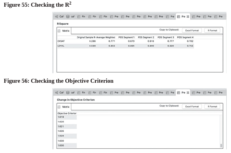
- Run the PLS-POS algorithm for a total of 10 times (i.e., repeat step 1 and 2 again for 9 more times) to avoid convergence on a local optimum. Choose the tab (run) that gives the highest value in terms of “R Square” and “Change in Objective Criterion”. That is, in each tab (run), go to the “Quality Criteria” heading to click the “R Square” and “Change in Objective Criterion” hyperlink respectively to compare their values.
- For example, in this PLS-POS calculation, the 7th run (tab) is the best solution because it gives the highest values of these model parameters (0.859 for R2 and 1.630 for Objective Criterion) among all runs (See Figure 55 and 56).
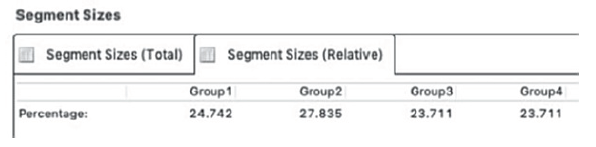
- Next, we go to “Final Results” heading and click the “Segment Sizes” hyperlink to check the segment size. Look at the 2nd tab for their relative segment sizes (see Figure 57):
- We build a table to summarize the findings in PLS-POS (see Figure 58): Figure 58: PLS-POS Model summary (R2)
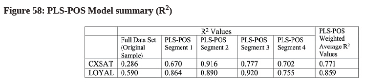
- From Figure 58, since the “PLS-POS Weighted Average R2 Values” are significantly larger than the “Full Dataset’s R2 Values”, we argue that a “4-segment” solution is preferred as it has higher predictive power than having a solution without segmentation.
- Becker et al., (2013) have stated that each segment should be differentiable. Using PLS-POS, we can test the significance of differences in path coefficients between segments. If a segment is not really different from one another, the researcher should consider combining it with another segment. To check the Path Coefficient, go to the “Final Results” heading and select “Path Coefficients”. Then, select the corresponding tab (e.g., Original Path Coefficient, POS Segment 1, POS Segment 2, POS Segment 3 and POS Segment 4) to view their respective path coefficients. Summarize the data in a table format (see Figure 59).
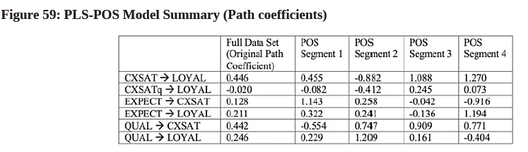
- It can be seen that in Segment 1, CXSAT has a positive impact on LOYAL (0.455) but CXSAT has a negative impact on LOYAL (-0.882) in Segment 2. Meanwhile, EXPECT has a positive impact on LOYAL in Segment 1, 2 and 4 but it has a negative impact on LOYAL (-0.136) in segment 3. It has also been observed that QUAL has a positive impact on LOYAL in segment 1, 2, and 3 but it has a negative impact on LOYAL (-0.404) in Segment 4.
- Once the PLS-POS results are generated, we can perform the ex-post analysis to interpret and characterize the segments obtained, using explanatory variables in the model/theory. In other words, we want to identify explanatory variables that match well with the PLS-POS partition.
7. Ex-post Analysis
- Open the “cafe100.csv” data file in Excel. Now, delete all observations with missing values. In this case, we have 3 observations with missing values, so our resulting dataset has 97 observations. Save this file as “cafe97.csv” and keep opening it in Excel.
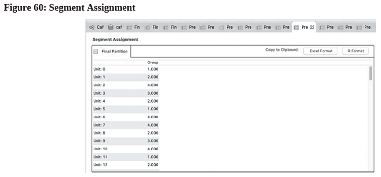
- In SmartPLS’ PLS-POS result page, go to the “Final Results” heading and click the “Segment Assignment” hyperlink.
- Press the “Excel Format” button59 on the right-hand side to copy the Final Partition information to the clipboard (see Figure 60).
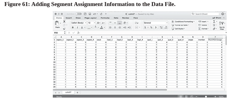
- Paste this data from clipboard to the next available column on the right-hand side of your data in the “cafe97.csv” file. Rename that column as “PLS-POS Groups” (see Figure 61):
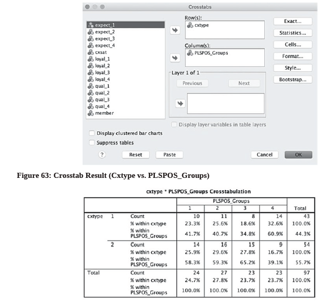
- Our goal is to compare the PLS-POS segments or partitions with those identified by other observable variables in the original dataset. Using statistical software like SPSS, import the data from this “cafe97.csv” file, and run a “Crosstab” analysis60 to show how these categories are related to each other.
- In our dataset, we have 2 observable variables; cxtype determines if the cafe patron is a student or not, whereas member determines if the cafe patron is a loyalty program member or not. We can compare them one by one.
- To begin with, we compare our PLS-POS Groups with cxtype in SPSS’ cross tab. (see Figure 62 & 63)
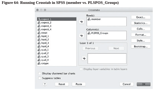
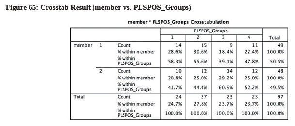
- Then, we compare our PLS-POS Groups with member in SPSS’ cross tab (see Figure 64 & 65).
- At this point, the researcher has to decide if the “number of segments” make any sense in reality. We want to ensure the retained segments are theoretically plausible.61 An important concept here is to turn unobserved heterogeneity into observed heterogeneity by making the segment accessible. This can be done by finding additional variables beyond the original model/theory to explain the plausible segments that are retained. Specifically, we may want to delete, add, or combine one or more segments for our subsequent analysis.
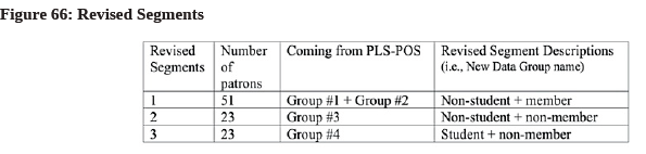
- From both Figure 63 and Figure 65, it can be seen that Group #1 and #2 are very similar in terms of their “% within PLSPOS_Groups”, so perhaps we can consider combining them into a single segment and call it “Segment 1”. The majority of this combined segment (with 51 cafe patrons) are non-students and member of the loyalty program.
- For Group #3, most cafe patrons are non-students (65.2%) and non-member of the loyalty program (60.9%). Meanwhile, most cafe patrons in Group #4 are students (60.9%) and non-members (52.2%)—. We can summarize these findings in the following Figure 66:
- Now, go back to SmartPLS to set up new data groups for PLS-SEM estimation. Recall that we now have a new dataset with only 97 observations, so we go to the “Project Explorer” tab and right click the blue-color “cafe100” icon. In the pop-up window, select the “cafe97.csv” data file and press OK. This “cafe97 [97 records]” file should now be highlighted.
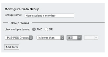
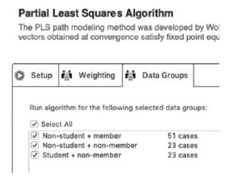
- Click the “Add Data Group” icon at the top. A new window called “Configure Data Group” appears. Type “Non-student + member” in the “Group Name:” box and set “PLS-POS Groups” is lower than 3, as in Figure 67, and then press “OK”.
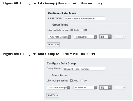
- Following the same process, create the other 2 new segments (see Figure 68 & 69).
- The final step is segment-specific model estimation. Assuming we are satisfied with the defined Data Groups, we can proceed to estimate the PLS path model for each data group separately. First, click the colorful model tab, then go to the “Calculate” menu and select “PLS Algorithm”. In the “Data Groups” tab, select the corresponding groups and start calculation (see Figure 70).
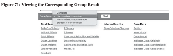
- In the “Data Group:” pull-down menu, select the first group called “Non-student + member”. Do not press the “next” button or else you will be viewing the next group’s result (see Figure 71).
- We also need to separately run bootstrapping for each segment and then compare path coefficient between them. That means click the colorful model tab, go to the “Calculate” menu and perform a “Bootstrapping” procedure using the default setting parameters. Assuming you have selected all groups in the “Data Group” tab, this bootstrapping procedure will be carried out for all segments simultaneously.
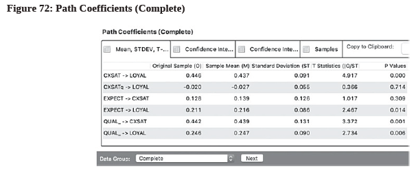
- The “Original Sample (O)” column shows the path coefficients for the aggregate model under the “Data Group: Complete” setting (see Figure 72).
- Select other segments in the pull-down menu to view their path coefficients.
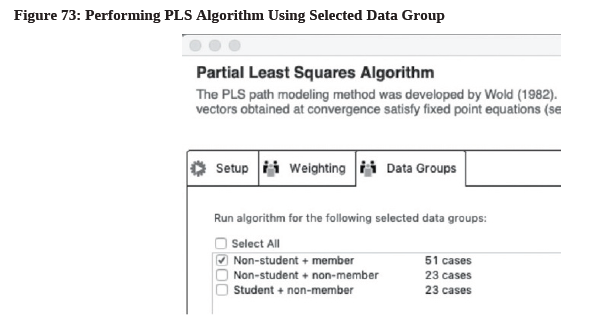
- Once that is done, check the R2 for these 3 newly formed segments. To do this, first click the colorful model tab. Go to the “Calculate” menu and select “PLS Algorithm”. In the Data Groups tab, only select the first group “Non-student + member”. Press “Start Calculation” (see Figure 73).
- Repeat this PLS Algorithm process one-by-one for the remaining 2 segments to get the R2. We can also calculate the weighted R2 by considering the group’s relative segment size.63 Since we make use of the reflective measurement model type64, we should also check the model’s (i) Convergent validity (AVE), (ii) Reliability (composite reliability, Cronbach’s alpha, rho_A), and (iii) Discriminant validity (HTMTinference). Summarize the data in a table like the one in Figure 74.
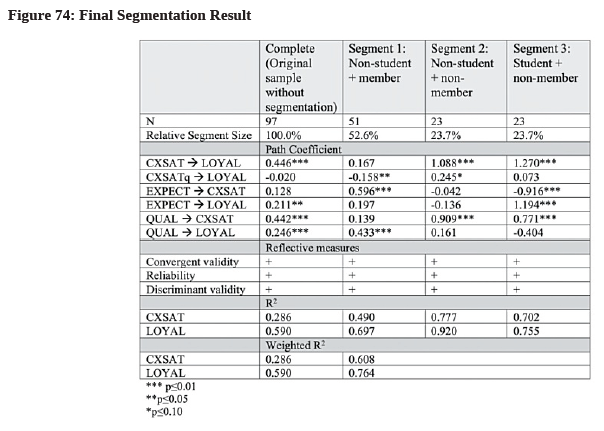
- From Figure 74, it can be seen that the weighted R2 (0.608 and 0.764) are larger than the original R2 for both CXSAT (0.286) and LOYAL (0.590) respectively. This clearly illustrates that grouping the data using the chosen explanatory variables increases the model’s in-sample predictive power, as compared to the aggregate, combined level analysis.
Comparing the path coefficients among the 3 segments in Figure 74, it is obvious that these segments are different in terms of their structural model effects. For example, the most important factor that leads to customer loyalty is QUAL (0.433, p<0.01) for segment 1. However, it is CXSAT that drives loyalty the most in
segment 2 (1.088, p<0.01) and segment 3 (1.270, p<0.01) respectively. Meanwhile, in the original homogenous sample, EXPECT has a significant effect on LOYAL (0.211, p<0.05), but the same can only be said for segment 3 (1.194, p<0.01) and not in segment 1 or 2. This completes the segment-specific model estimation.
- Using these results, the cafe owner can draw some managerial implications. For example, about half of the patrons being surveyed hold loyalty card membership and this customer segment cares more about perceived quality (QUAL) than other aspects of the business. Hence, the cafe owner should prioritize to ensure it has tasty food, friendly servers, accurate billing, and well-crafted drinks. On the other hand, if the cafe owner believes that students play a strategic role in the future growth of her cafe, she need to focus on improving customer expectation (EXPECT) because it is the second most important factor in driving loyalty after customer satisfaction (CXSAT). That is, the owner should make sure her cafe has best menu selection, great atmospheric elements, good looking servers and affordable daily specials.
- In the ideal scenario, marketing researcher should consider validating their segmentation results with other data that are not used in the estimation process, and/or repeating the segmentation analysis on another population. By using external data or collecting addition data in a follow-up study, researcher can test the proposed explanatory variables to make the research results more generalizable with the ultimate goal of refining the theory.
Source: Ken Kwong-Kay Wong (2019), Mastering Partial Least Squares Structural Equation Modeling (Pls-Sem) with Smartpls in 38 Hours, iUniverse.
28 Sep 2021
28 Sep 2021
28 Sep 2021
28 Sep 2021
28 Sep 2021
28 Sep 2021