Comparisons among r, g, and o

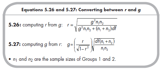
I have emphasized the importance of basing the decision to rely on r, g, or o on conceptualizations of the association involving two continuous vari­ables, a dichotomous and a continuous variable, or two dichotomous vari­ables, respectively. At the same time, it can be useful to understand that you can compute values of one effect size from values of another effect size. For example, r and g can be computed from one another using the following formulas:

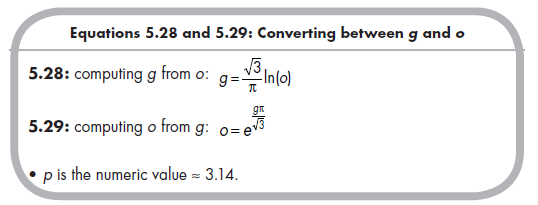
Similarly, g and o can be computed from one another using the following equations:

Finally, you can transform from o to r by reconstructing the contingency table (if sufficient information is provided), through intermediate transfor­mations to g, or through one of several approximations of the tetrachoric cor­relation (see Bonett, 2007). An intermediate transformation to g or algebraic rearrangement of the tetrachoric correlation approximations also allows you to transform from r to o.

This mathematical interchangeability among effect sizes has led to arguments that one type of effect size is preferable to another. For example, Rosenthal (1991) has expressed preference for r over d (and presumably other standardized mean differences, including g) based on four features. First, comparisons of Equations 5.13 and 5.14 for r versus 5.20 and 5.21 for g reveal that it is possible to compute r accurately from only the inferential test value and degrees of freedom, whereas computing g requires knowing the group sample sizes or else approximating this value by assuming that the group sizes are equal. To the extent that primary studies do not report group sizes and it is reasonable to expect marked differences in group sizes, r is prefer­able to d. A second, smaller, argument for preferring r to g is that you use the same equations to compute r from independent sample versus repeated- measures inferential tests, whereas different formulas are necessary when computing g from these tests (see Equations 5.20 and 5.21 vs. 5.22). This should not pose too much difficulty for the competent meta-analyst, but con­sideration of simplicity is not trivial. A third advantage of r over standardized mean differences, according to Rosenthal (1991), is in ease of interpretation. Whether r or standardized mean differences (e.g., g) are more intuitive to readers is debatable and currently is a matter of opinion rather than care­ful study. It probably is the case that most scientists have more exposure to r than to g or d, but this does not mean that they cannot readily grasp the meaning of the standardized mean difference. The final, and perhaps most convincing, argument for Rosenthal’s (1991) preference is that r can be used whenever d can (e.g., in describing an association between a dichotomous variable and a continuous variable), but it makes less sense to use g in many situations where r could be used (e.g., in describing an association between two continuous variables).

Arguments have also been put forth for preferring o to standardized mean differences (g or d) or r when both variables are truly dichotomous. The magnitudes of r (typically denoted with ^) or standardized mean differ­ences (g or d) that you can compute from a 2 X 2 contingency table depend on the marginal frequencies of the dichotomies. This dependence leads to attenuated effect sizes as well as extraneous heterogeneity among studies when these effect size indices are used with dichotomous data (Fleiss, 1994; Haddock et al., 1998). This limitation is not present for o, leading many to argue that it is the preferred effect size to index associations between dichotomous data.

I do not believe that any type of effect size index (i.e., r, g, or o) is inher­ently preferable to another. What is far more important is that you select the effect size that matches your conceptualization of the variables under con­sideration. Linear associations between two variables that are naturally con­tinuous should be represented with r. Associations between a dichotomous variable (e.g., group) and a continuous variable can be represented with a standardized mean difference (e.g., g) or r, with a standardized mean differ­ence probably more naturally representing this type of association.¹⁴ Asso­ciations between two natural dichotomies are best represented with o.

If you wish to compare multiple levels of variables in the same meta­analysis, I recommend using the effect size index representing the more con­tinuous nature for both. For example, associations of a continuous variable (e.g., aggressive) with a set of correlates that includes a mixture of continuous and dichotomous variables (e.g., a continuous rejection variable and a dichot­omous variable of being classified as rejected) could be well represented with the correlation coefficient, r (Rosenthal, 1991). Similarly, associations of a dichotomous variable (e.g., biological sex) with a set containing a combina­tion of continuous (e.g., rejection) and dichotomous (e.g., rejection classifi­cation) variables could be represented with a standardized mean difference such as g (Sanchez-Meca et al., 2003). In both cases, it would be important to evaluate moderation by the type (i.e., continuous versus dichotomous) of correlate.

Source: Card Noel A. (2015), Applied Meta-Analysis for Social Science Research, The Guilford Press; Annotated edition.