Conditional Probability

Often, the probability of an event is influenced by whether a related event already occurred. Suppose we have an event A with probability P(A). If we obtain new information and learn that a related event, denoted by B, already occurred, we will want to take advantage of this information by calculating a new probability for event A. This new probability of event A is called a conditional probability and is written P(A I B). We use the notation I to indicate that we are considering the probability of event A given the condition that event B has occurred. Hence, the notation P(A I B) reads “the probability of A given B ”

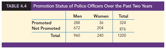
As an illustration of the application of conditional probability, consider the situation of the promotion status of male and female officers of a major metropolitan police force in the eastern United States. The police force consists of 1200 officers, 960 men and 240 women. Over the past two years, 324 officers on the police force received promotions. The specific breakdown of promotions for male and female officers is shown in Table 4.4.

After reviewing the promotion record, a committee of female officers raised a discrimination case on the basis that 288 male officers had received promotions, but only 36 female officers had received promotions. The police administration argued that the relatively low number of promotions for female officers was due not to discrimination, but to the fact that relatively few females are members of the police force. Let us show how conditional probability could be used to analyze the discrimination charge.

Let

M = event an officer is a man

W = event an officer is a woman

A = event an officer is promoted

A^c = event an officer is not promoted

Dividing the data values in Table 4.4 by the total of 1200 officers enables us to summarize the available information with the following probability values.

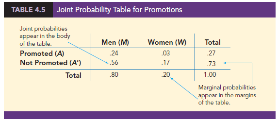
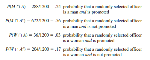
Because each of these values gives the probability of the intersection of two events, the probabilities are called joint probabilities. Table 4.5, which provides a summary of the probability information for the police officer promotion situation, is referred to as a joint probability table.

The values in the margins of the joint probability table provide the probabilities of each event separately. That is, P(M) = .80, P(W) = .20, P(A) = .27, and P(Ac) = .73. These probabilities are referred to as marginal probabilities because of their location in the margins of the joint probability table. We note that the marginal probabilities are found by summing the joint probabilities in the corresponding row or column of the joint probability table. For instance, the marginal probability of being promoted is P(A) = P(M ∩ A) + P(W ∩ A) = .24 + .03 = .27. From the marginal probabilities, we see that 80% of the force is male, 20% of the force isfemale, 27% of all officers received promotions, and 73% were not promoted.

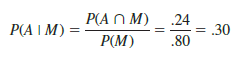
Let us begin the conditional probability analysis by computing the probability that an officer is promoted given that the officer is a man. In conditional probability notation, we are attempting to determine P(A I M). To calculate P(A I M), we first realize that this notation simply means that we are considering the probability of the event A (promotion) given that the condition designated as event M (the officer is a man) is known to exist. Thus P(A I M) tells us that we are now concerned only with the promotion status of the 960 male officers. Because 288 of the 960 male officers received promotions, the probability of being promoted given that the officer is a man is 288/960 = .30. In other words, given that an officer is a man, that officer had a 30% chance of receiving a promotion over the past two years.

This procedure was easy to apply because the values in Table 4.4 show the number of officers in each category. We now want to demonstrate how conditional probabilities such as P(A I M) can be computed directly from related event probabilities rather than the frequency data of Table 4.4.

We have shown that P(A I M) = 288/960 = .30. Let us now divide both the numerator and denominator of this fraction by 1200, the total number of officers in the study.

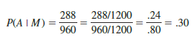
We now see that the conditional probability P(A I M) can be computed as .24/.80. Refer to the joint probability table (Table 4.5). Note in particular that .24 is the joint probability of A and M; that is, P(A n M) = .24. Also note that .80 is the marginal probability that a randomly selected officer is a man; that is, P(M) = .80. Thus, the conditional probability P(A I M) can be computed as the ratio of the joint probability P(A n M) to the marginal probability P(M).

The fact that conditional probabilities can be computed as the ratio of a joint probability to a marginal probability provides the following general formula for conditional probability calculations for two events A and B.

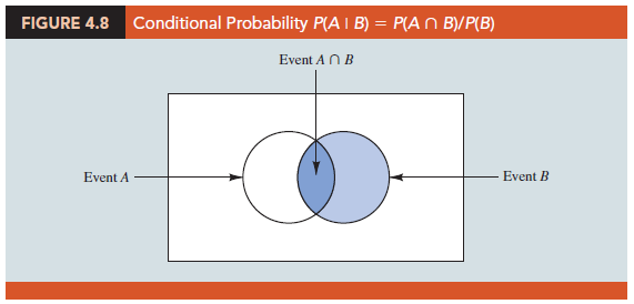
The Venn diagram in Figure 4.8 is helpful in obtaining an intuitive understanding of conditional probability. The circle on the right shows that event B has occurred; the portion of the circle that overlaps with event A denotes the event (A n B). We know that once event B has occurred, the only way that we can also observe event A is for the event (A n B) to occur. Thus, the ratio P(A n B)/P(B) provides the conditional probability that we will observe event A given that event B has already occurred.

Let us return to the issue of discrimination against the female officers. The marginal probability in row 1 of Table 4.5 shows that the probability of promotion of an officer is P(A) = .27 (regardless of whether that officer is male or female). However, the critical issue in the discrimination case involves the two conditional probabilities P(A I M) and P(A I W). That is, what is the probability of a promotion given that the officer is a man, and what is the probability of a promotion given that the officer is a woman? If these two probabilities are equal, a discrimination argument has no basis because the chances of a promotion are the same for male and female officers. However, a difference in the two conditional probabilities will support the position that male and female officers are treated differently in promotion decisions.

We already determined that P(A I M) = .30. Let us now use the probability values in Table 4.5 and the basic relationship of conditional probability in equation (4.7) to compute the probability that an officer is promoted given that the officer is a woman; that is, P(A I W). Using equation (4.7), with W replacing B, we obtain

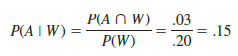
What conclusion do you draw? The probability of a promotion given that the officer is a man is .30, twice the .15 probability of a promotion given that the officer is a woman. Although the use of conditional probability does not in itself prove that discrimination exists in this case, the conditional probability values support the argument presented by the female officers.

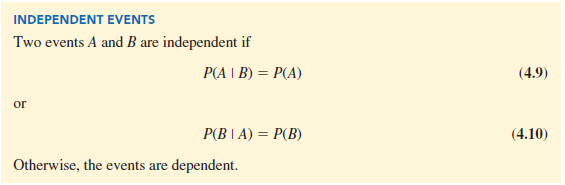
1. Independent Events

In the preceding illustration, P(A) = .27, P(A I M) = .30, and P(A I W) = .15. We see that the probability of a promotion (event A) is affected or influenced by whether the officer is a man or a woman. Particularly, because P(A I M) A P(A), we would say that events A and M are dependent events. That is, the probability of event A (promotion) is altered or affected by knowing that event M (the officer is a man) exists. Similarly, with P(A I W) A P(A), we would say that events A and W are dependent events. However, if the probability of event A is not changed by the existence of event M—that is, P(A I M) = P(A)—we would say that events A and M are independent events. This situation leads to the following definition of the independence of two events.

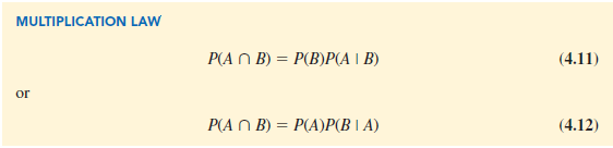
2. Multiplication Law

Whereas the addition law of probability is used to compute the probability of a union of two events, the multiplication law is used to compute the probability of the intersection of two events. The multiplication law is based on the definition of conditional probability. Using equations (4.7) and (4.8) and solving for P(A fl B), we obtain the multiplication law.

To illustrate the use of the multiplication law, consider a telecommunications company that offers services such as high-speed Internet, cable television, and telephone services. For a particular city, it is known that 84% of the households subscribe to high-speed Internet service. If we let H denote the event that a household subscribes to high-speed Internet service, P(H) = .84. In addition, it is known that the probability that a household that already subscribes to high-speed Internet service also subscribes to cable television service (event C) is .75; that is, P(C I H) = .75. What is the probability that a household subscribes to both high-speed Internet and cable television services? Using the multiplication law, we compute the desired P(C fl H) as

We now know that 63% of the households subscribe to both high-speed Internet and cable television services.

Before concluding this section, let us consider the special case of the multiplication law when the events involved are independent. Recall that events A and B are independent whenever P(A I B) = P(A) or P(B I A) = P(B). Hence, using equations (4.11) and (4.12) for the special case of independent events, we obtain the following multiplication law.

To compute the probability of the intersection of two independent events, we simply multiply the corresponding probabilities. Note that the multiplication law for independent events provides another way to determine whether A and B are independent. That is, if P(A f B) = P(A)P(B), then A and B are independent; if P(A f B) A P(A)P(B), then A and B are dependent.

As an application of the multiplication law for independent events, consider the situation of a service station manager who knows from past experience that 80% of the customers use a credit card when they purchase gasoline. What is the probability that the next two customers purchasing gasoline will each use a credit card? If we let

A = the event that the first customer uses a credit card

B = the event that the second customer uses a credit card

then the event of interest is A f B. Given no other information, we can reasonably assume that A and B are independent events. Thus,

To summarize this section, we note that our interest in conditional probability is motivated by the fact that events are often related. In such cases, we say the events are dependent and the conditional probability formulas in equations (4.7) and (4.8) must be used to compute the event probabilities. If two events are not related, they are independent; in this case neither event’s probability is affected by whether the other event occurred.

Source: Anderson David R., Sweeney Dennis J., Williams Thomas A. (2019), Statistics for Business & Economics, Cengage Learning; 14th edition.