Bayes’ Theorem

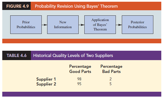
In the discussion of conditional probability, we indicated that revising probabilities when new information is obtained is an important phase of probability analysis. Often, we begin the analysis with initial or prior probability estimates for specific events of interest. Then, from sources such as a sample, a special report, or a product test, we obtain additional information about the events. Given this new information, we update the prior probability values by calculating revised probabilities, referred to as posterior probabilities. Bayes’ theorem provides a means for making these probability calculations. The steps in this probability revision process are shown in Figure 4.9.

As an application of Bayes’ theorem, consider a manufacturing firm that receives shipments of parts from two different suppliers. Let A₁ denote the event that a part is from supplier 1 and A₂ denote the event that a part is from supplier 2. Currently, 65% of the parts purchased by the company are from supplier 1 and the remaining 35% are from supplier 2. Hence, if a part is selected at random, we would assign the prior probabilities P(A₁) = .65 and P(A₂) = .35.

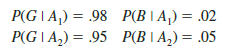
The quality of the purchased parts varies with the source of supply. Historical data suggest that the quality ratings of the two suppliers are as shown in Table 4.6. If we let G denote the event that a part is good and B denote the event that a part is bad, the informa­tion in Table 4.6 provides the following conditional probability values.

The tree diagram in Figure 4.10 depicts the process of the firm receiving a part from one of the two suppliers and then discovering that the part is good or bad as a two-step experiment. We see that four experimental outcomes are possible; two correspond to the part being good and two correspond to the part being bad.

Each of the experimental outcomes is the intersection of two events, so we can use the multiplication rule to compute the probabilities. For instance,

The process of computing these joint probabilities can be depicted in what is called a probability tree (see Figure 4.11). From left to right through the tree, the probabilities for each branch at step 1 are prior probabilities and the probabilities for each branch at step 2 are conditional probabilities. To find the probabilities of each experimental outcome, we simply multiply the probabilities on the branches leading to the outcome. Each of these joint proba­bilities is shown in Figure 4.11 along with the known probabilities for each branch.

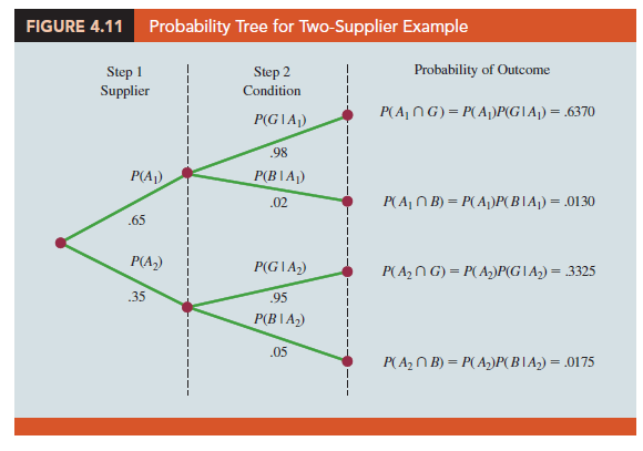
Suppose now that the parts from the two suppliers are used in the firm’s manufac­turing process and that a machine breaks down because it attempts to process a bad part. Given the information that the part is bad, what is the probability that it came from supplier 1 and what is the probability that it came from supplier 2? With the information in the probability tree (Figure 4.11), Bayes’ theorem can be used to answer these questions.

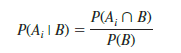
Letting B denote the event that the part is bad, we are looking for the posterior probabil­ities P(A₁ I B) and P(A₂ I B). From the law of conditional probability, we know that

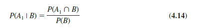
Referring to the probability tree, we see that

To find P(B), we note that event B can occur in only two ways: (A₁ n B) and (A₂ n B). Therefore, we have

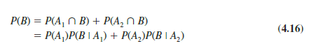
Substituting from equations (4.15) and (4.16) into equation (4.14) and writing a similar result for P(A2 ∣ B), we obtain Bayes’ theorem for the case of two events.

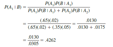
Using equation (4.17) and the probability values provided in the example, we have

In addition, using equation (4.18), we find P(A₂ I B).

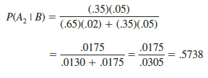
Note that in this application we started with a probability of .65 that a part selected at ran­dom was from supplier 1. However, given information that the part is bad, the probability that the part is from supplier 1 drops to .4262. In fact, if the part is bad, it has better than a 50-50 chance that it came from supplier 2; that is, P(A₂ I B) = .5738.

Bayes’ theorem is applicable when the events for which we want to compute posterior probabilities are mutually exclusive and their union is the entire sample space.^[1] For the case of n mutually exclusive events A₁, A₂, . . . , A_n, whose union is the entire sample space, Bayes’ theorem can be used to compute any posterior probability P(A, I B) as shown here.

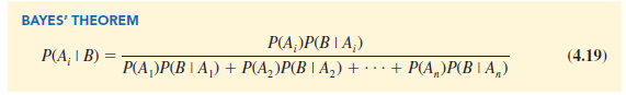
With prior probabilities P(A₁), P(A₂), . . . , P(A_n) and the appropriate conditional probabili­ties P(B I A₁), P(B I A₂), . . . , P(B I A_n), equation (4.19) can be used to compute the poste­rior probability of the events A₁, A₂, . . . , A_n.

1. Tabular Approach

A tabular approach is helpful in conducting the Bayes’ theorem calculations. Such an approach is shown in Table 4.7 for the parts supplier problem. The computations shown there are done in the following steps.

Step 1. Prepare the following three columns:

Column 1—The mutually exclusive events A_i for which posterior probabilities are desired

Column 2—The prior probabilities P(A_i) for the events

Column 3—The conditional probabilities P(B I A) of the new information B given each event

Step 2. In column 4, compute the joint probabilities P(A_i Cl B) for each event and the new information B by using the multiplication law. These joint probabili­ties are found by multiplying the prior probabilities in column 2 by the corresponding conditional probabilities in column 3; that is, P(A, C B) = P(A)P(B I A,.).

Step 3. Sum the joint probabilities in column 4. The sum is the probability of the new information, P(B). Thus we see in Table 4.7 that there is a .0130 probability that the part came from supplier 1 and is bad and a .0175 probability that the part came from supplier 2 and is bad. Because these are the only two ways in which a bad part can be obtained, the sum .0130 + .0175 shows an overall probability of .0305 of finding a bad part from the combined shipments of the two suppliers.

Step 4. In column 5, compute the posterior probabilities using the basic relationship of conditional probability.

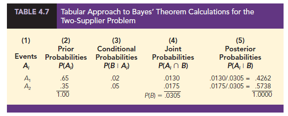
Note that the joint probabilities P(A_t n B) are in column 4 and the probability P(B) is the sum of column 4.

Source:  Anderson David R., Sweeney Dennis J., Williams Thomas A. (2019), Statistics for Business & Economics, Cengage Learning; 14th edition.