Some Basic Relationships of Probability

Given an event A, the complement of A is defined to be the event consisting of all sample points that are not in A. The complement of A is denoted by A^c. Figure 4.4 is a diagram, known as a Venn diagram, which illustrates the concept of a complement. The rectangular area represents the sample space for the experiment and as such contains all possible sample points. The circle represents event A and contains only the sample points that belong to A. The shaded region of the rectangle contains all sample points not in event A and is by definition the complement of A.

In any probability application, either event A or its complement A^c must occur. Therefore, we have

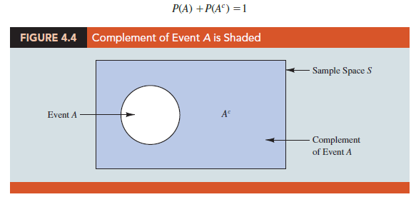
Solving for P(A), we obtain the following result.

Equation (4.5) shows that the probability of an event A can be computed easily if the probability of its complement, P(A^c), is known.

As an example, consider the case of a sales manager who, after reviewing sales reports, states that 80% of new customer contacts result in no sale. By allowing A to denote the event of a sale and A^c to denote the event of no sale, the manager is stating that P(A^c) = .80. Using equation (4.5), we see that

We can conclude that a new customer contact has a .20 probability of resulting in a sale.

In another example, a purchasing agent states a .90 probability that a supplier will send a shipment that is free of defective parts. Using the complement, we can conclude that there is a 1 – .90 = .10 probability that the shipment will contain defective parts.

1. Addition Law

The addition law is helpful when we are interested in knowing the probability that at least one of two events occurs. That is, with events A and B we are interested in knowing the probability that event A or event B or both occur.

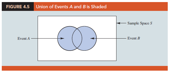
Before we present the addition law, we need to discuss two concepts related to the com­bination of events: the union of events and the intersection of events. Given two events A and B, the union of A and B is defined as follows.

The Venn diagram in Figure 4.5 depicts the union of events A and B. Note that the two circles contain all the sample points in event A as well as all the sample points in event B. The fact that the circles overlap indicates that some sample points are contained in both A and B.

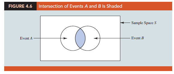
The Venn diagram depicting the intersection of events A and B is shown in Figure 4.6. The area where the two circles overlap is the intersection; it contains the sample points that are in both A and B.

Let us now continue with a discussion of the addition law. The addition law provides a way to compute the probability that event A or event B or both occur. In other words, the addition law is used to compute the probability of the union of two events. The addition law is written as follows.

To understand the addition law intuitively, note that the first two terms in the addition law, P(A) + P(B), account for all the sample points in A U B. However, because the sample points in the intersection A n B are in both A and B, when we compute P(A) + P(B), we are in effect counting each of the sample points in A n B twice. We correct for this overcounting by subtracting P(A n B).

As an example of an application of the addition law, let us consider the case of a small assembly plant with 50 employees. Each worker is expected to complete work assign­ments on time and in such a way that the assembled product will pass a final inspection. On occasion, some of the workers fail to meet the performance standards by completing work late or assembling a defective product. At the end of a performance evaluation period, the production manager found that 5 of the 50 workers completed work late, 6 of the 50 workers assembled a defective product, and 2 of the 50 workers both completed work late and assembled a defective product.

Let

L = the event that the work is completed late

D = the event that the assembled product is defective

The relative frequency information leads to the following probabilities.

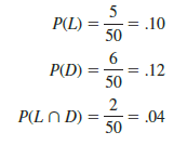
After reviewing the performance data, the production manager decided to assign a poor performance rating to any employee whose work was either late or defective; thus the event of interest is L U D. What is the probability that the production manager assigned an employee a poor performance rating?

Note that the probability question is about the union of two events. Specifically, we want to know P(L U D). Using equation (4.6), we have

Knowing values for the three probabilities on the right side of this expression, we can write

This calculation tells us that there is a .18 probability that a randomly selected employee received a poor performance rating.

As another example of the addition law, consider a recent study conducted by the personnel manager of a major computer software company. The study showed that 30% of the employees who left the firm within two years did so primarily because they were dissatisfied with their salary, 20% left because they were dissatisfied with their work assignments, and 12% of the former employees indicated dissatisfaction with both their salary and their work assignments. What is the probability that an employee who leaves within two years does so because of dissatisfaction with salary, dissatisfaction with the work assignment, or both?

Let

S 5 the event that the employee leaves because of salary

W 5 the event that the employee leaves because of work assignment

We have P(S) = .30, P(W) = .20, and P(S fl W) = .12. Using equation (4.6), the addition law, we have

P(S U W) 5 P(S) + P(W) – P(S n W) 5 .30 + .20 – .12 5 .38.

We find a .38 probability that an employee leaves for salary or work assignment reasons.

Before we conclude our discussion of the addition law, let us consider a special case that arises for mutually exclusive events.

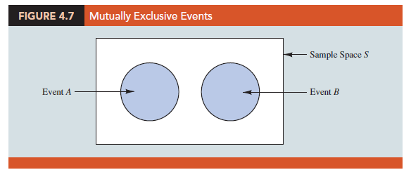
MUTUALLY EXCLUSIVE EVENTS

Two events are said to be mutually exclusive if the events have no sample points in common.

Events A and B are mutually exclusive if, when one event occurs, the other cannot occur. Thus, a requirement for A and B to be mutually exclusive is that their intersection must contain no sample points. The Venn diagram depicting two mutually exclusive events A and B is shown in Figure 4.7. In this case P(A f B) = 0 and the addition law can be written as follows.

Source:  Anderson David R., Sweeney Dennis J., Williams Thomas A. (2019), Statistics for Business & Economics, Cengage Learning; 14th edition.