Cross-Sectional Time Series by using Stata

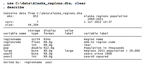
This section applies xtmixed to a different kind of multilevel data: cross-sectional time series. Dataset Alaskaregions.dta contains time series of population for each of the 27 boroughs, municipalities or census areas that together make up the state of Alaska. These 27 regions are a fragment from the pan-Arctic human-dimensions database framework described by Hamilton and Lammers (2011). In Alaska regions.dta, a dummy variable named large marks the five most populous Alaska regions, those having 2011 populations greater than 20,000. The other 22 regions are predominantly rural, and their smaller populations might be widely dispersed. The Northwest Arctic borough, for example, covers a geographic area larger than the state of Maine, but had a 2011 population of fewer than 8,000 people. For each of the 27 regions there are multiple years of data, ranging from 1969 to 2011 but with many missing values. Thus, for each variable there are 27 parallel but often incomplete time series.

During the first half of the time period covered by these data, population grew substantially in many parts of rural Alaska. In more recent years, however, the rate of growth leveled off, and populations in some areas declined. The trends are relevant to discussions about sustainable economic development for these places, and also for their cultural importance to the Alaska Native populations who live there.

Because population trends have not simply gone upwards, they cannot realistically be modeled as a linear function of year. The mixed model below represents population trends as a quadratic function, regressing population in thousands (pop) on years since 1968 (year0) and also on year0 squared. We allow for fixed (/() and random (u ) intercepts and slopes on both terms. The 5 large-population regions are set aside for these analysis, in order to focus on rural Alaska.

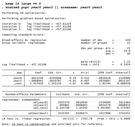
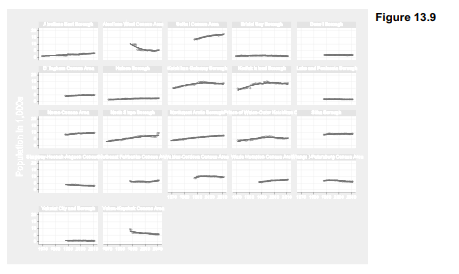
All the random effects show significant variation from place to place. The fixed-effect coefficients on yearO and year2, on the other hand, do not differ significantly from zero — indicating the lack of an overall trend across these 22 regions. Graphing predicted population (with a median-spline curve) and actual population against calendar year helps to visualize the details of area-to-area variation and why xtmixed finds no overall trend (Figure 13.9). In some areas the population grew steadily, while in others the direction of growth or decline reversed. The model does a decent job of smoothing past some visible discontinuities in the data, such as the Aleutians West population drop that followed downsizing of a naval air station in 1994, or the North Slope gain that followed inclusion of employees at remote work sites in the 2010 Census.

. predict yhat, fitted

. graph twoway scatter pop year, msymbol(Oh)

|| mspline yhat year, lwidth(medthick) bands(50)

|| , by(regionname, note(“”) legend(off))

ylabel(0(5)20, angle(horizontal))

xtitle(“”) ytitle(“Population in 1,000s”)

xlabel(1970(10)2010, grid)

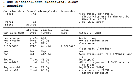
A more substantive analysis using mixed-effects regression to model relationships involving multiple time series appears in a paper on population, climate and electricity use in towns and villages of Arctic Alaska (Hamilton et al. 2011). Dataset Alaska_places.dta contains the core data for this analysis, consisting of annual time series for each of 42 towns and villages in Arctic Alaska, all within five of the census regions or boroughs graphed in Figure 13.9 above. Variables include community population, kilowatt hours of electricity sold, the average rate charged for electricity (in constant 2009 dollars), and estimates of the summer temperature and precipitation around that location each year. The paper supplies information about variable definitions, data sources and the context for this analysis.

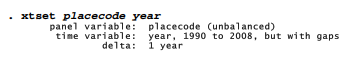
These data have been declared as panel through an xtset command that specified placecode as the panel variable and year as the time variable:

The mixed-effect analysis below models the kilowatt hours of electricity sold in each community, each year, as a function of population, electricity rate in constant 2009 dollars, summer temperature and precipitation, and year. The model includes random effects for population, and first-order autoregressive errors. Reasoning behind this particular specification, and tests for the robustness of modeling results, are given in the paper; the short presentation here just aims to show what such an analysis looks like.

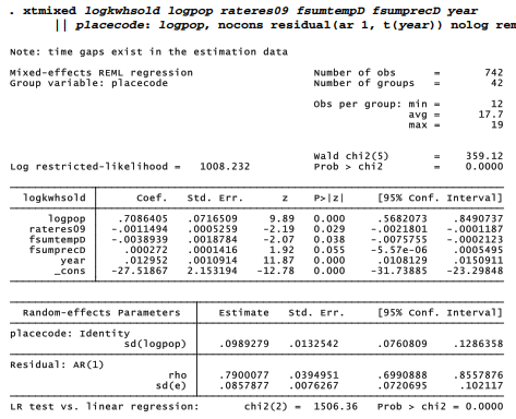
Electricity use in these Arctic towns and villages is predicted by population, price and summer temperature. Unlike lower latitudes where warm summers often mean more electricity use for air conditioning, in these Arctic places warmer (and often, less rainy) summers can encourage people to spend more time outdoors. Adjusting for the effects of population, price and weather, we see an overall upward trend in use as life became more electricity-intensive. Finally, significant variation in the random slope on population indicates that the per-person effects differ from place to place. They tend to be largest in the most northerly region, communities of the North Slope Borough. The autoregressive AR(1) error term proves statistically significant as well.

As noted in Chapter 12, time series often are tested for stationarity before modeling, to avoid reaching spurious conclusions. Differencing provides one set oftools. Alternatively, even when the original series are nonstationary, as in this example (or the ARMAX models in Chapter 12), we can seek a linear combination of the variables that is stationary (cotntegration; see Hamilton 1994). Model [13.8] serves well for this purpose. None of the 42 residual series (one series for each community) generated by this model show significant autocorrelation, as tested by Ljung- Box portmanteau Q statistics. Thus, residuals are not distinguishable from white noise, a covariance stationary process. The following commands calculate predicted values taking the autoregressive term into account (yhat xt), then use those predictions to calculate residuals (restdxt). White-noise Q tests (wntestq) showing no residual autocorrelation are illustrated below for the first 3 out of 42 communities.

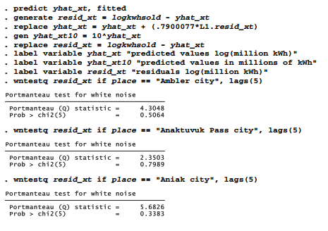
Similar tests for all 42 communities found that none of the residual series exhibited significant autocorrelation.

Source: Hamilton Lawrence C. (2012), Statistics with STATA: Version 12, Cengage Learning; 8th edition.