Exploratory Data Analysis by using Stata

Statistician John Tukey assembled a toolkit of old and new methods for exploratory data analysis (EDA), which involves analyzing data in an exploratory and skeptical way without making unneeded assumptions (see Tukey 1977; also Hoaglin, Mosteller and Tukey 1983, 1985). Box plots, introduced in Chapter 3, are one the most popular EDA methods. Another is the stem-and-leaf display, a graphical arrangement of ordered data values in which initial digits form the stems and following digits for each observation make up the leaves.

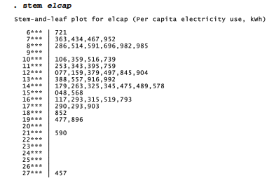
In this display the lowest per capita electricity value, 6,721 (California), appears as a 721 leaf on the 6*** stem. The highest, 27,457 (Wyoming), appears as a 457 leaf on the 27*** stem. stem automatically chooses values for the stems, but can override this with a lines( ) option. Type help stem for information about this option and others.

Letter-value displays (lv) use order statistics to dissect a distribution.

M denotes the median, and F the “fourths” (quartiles, using a different approximation than the quartile approximation used by summarize, detail and tabsum). E , D , C , . . . denote cutoff points such that roughly 1/8, 1/16, 1/32, . . . of the distribution remains outside in the tails. The second column of numbers gives the depth or distance from the nearest extreme, for each letter value. Within the center box, the middle column gives midsummaries, which are averages of the two letter values. If midsummaries drift away from the median, as they do for elcap, this tells us that the distribution becomes progressively more skewed as we move farther out into the tails. The spreads are differences between pairs of letter values. For instance, the spread between Fs equals the approximate interquartile range. Finally, pseudosigmas in the right-hand column estimate what the standard deviation should be if these letter values described a Gaussian
population. The F pseudosigma, sometimes called a pseudo standard deviation (PSD), provides a simple and outlier-resistant check for approximate normality in symmetrical distributions:

1. Comparing mean with median diagnoses overall skew:

mean > median                      positive skew

mean = median                      symmetry

mean < median                      negative skew

2. If the mean and median are similar, indicating symmetry, then a comparison between standard deviation and PSD helps to evaluate tail normality:

standard deviation > PSD heavier-than-normal tails

standard deviation = PSD normal tails

standard deviation < PSD lighter-than-normal tails

Let F₁ and F₃ denote 1st and 3rd fourths (approximate 25th and 75th percentiles).

Then the interquartile range, IQR, equals F₃ – F₁ , and PSD = IQR / 1.349.

lv also identifies mild and severe outliers, if any exist (there is only one mild outlier in the elcap distribution). We call an x value a “mild outlier” when it lies outside the inner fence, but not outside the outer fence:

F₁ – 3IQR < x < F₁ – 1.5IQR       or F₃ + 1.5IQR < x < F₃ + 3IQR

The value of x is a “severe outlier” if it lies outside the outer fence:

x < F₁ – 3IQR or x > F₃ + 3IQR

lv gives these cutoffs and the number of outliers of each type. Severe outliers, values beyond the outer fences, occur sparsely (about two per million) in normal populations. Monte Carlo simulations suggest that the presence of any severe outliers in samples of n = 15 to about 20,000 should be sufficient evidence to reject a normality hypothesis at α= .05 (Hamilton 1992b). Severe outliers create problems for many statistical techniques.

summarize, stem and lv all confirm that lived has a positively skewed sample distribution, not resembling a theoretical normal curve. The next section introduces more formal normality tests, and transformations that can reduce a variable’s skew.

Source: Hamilton Lawrence C. (2012), Statistics with STATA: Version 12, Cengage Learning; 8th edition.