Time series analysis often involves lagged variables, or values from previous times. Lags can be specified by explicit subscripting. For example, the following command creates variable mei l, equal to the previous month’s Multivariate ENSO Index (mei) value:
. generate mei_1 = mei[_n-1]
Alternatively, we could accomplish the same thing, using tsset data, with Stata’s L. (lag) operators. Lag operators are simpler than an explicit-subscripting approach. More importantly, the lag operators also respect panel data. The following commands generate 1- and 2-month lagged values of mei.

We could have obtained this same list without generating any new variables by typing
. list year month mei L1.mei L2.mei in -5/l
The L. operator is one of several that simplify working with time series datasets. Other time series operators are F. (lead), D. (difference) and S. (seasonal difference). These operators can be typed either in upper or lower case — for example, F2.mei or f2.mei.
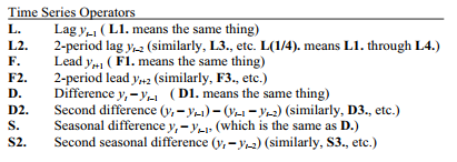
In the case of seasonal differences, S12. does not mean 12th difference, but rather a first difference at lag 12. For example, if we had actual global CO2 values instead of anomalies, we would see a clear seasonal pattern — lowest in August and September. For some purposes we might want to calculate S12.co2, which would be the differences between January 1981 co2 and January 1980 co2, February 1981 co2 and February 1980 co2, and so forth.
Lag operators can appear directly in most analytical commands involving tsset data. The following example regresses global temperature (ncdctemp) on the previous month’s Aerosol Optical Depth (aod) index, which in theory should exert a cooling effect. The regression is done without a need to create any new lagged variables.
. regress ncdctemp L1.aod
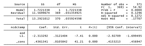
As expected, aod has a negative effect on global temperature. The estimated model involves monthly temperature as a function of the previous month’s aod:
predicted ncdctempt = .436 -2.313aodt-1
The coefficient on lagged aod (-2.313) appears to be statistically significant (p =0.000), but the standard errors and tests in this regression may not be valid. As with any OLS model, they depend on the assumption that errors for successive observations are independent or uncorrelated with each other. Correlated errors occur often in time series analysis, however, so we routinely test for their presence as done in the next section. Standard errors, confidence intervals and tests from OLS regressions involving time series should generally be viewed with suspicion, unless testing shows no evidence of correlated errors.
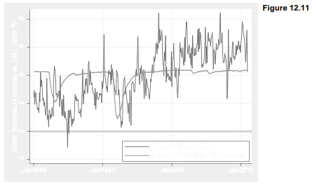
Although the possibility of correlated errors makes t and F tests from this regression untrustworthy, the regression equation itself can still provide a valid, least-squares description of the data. Figure 12.11 graphs the predicted values along with observed temperature. The giant Pinatubo eruption in 1991 predicts a substantial cooling, which does appear in the temperature data. Obviously, however, there is much more besides these two volcanoes affecting global climate.
Continuing for the moment in a purely descriptive mode, we could explore whether other proposed temperature drivers in these data improve the fit to observed temperatures. Including lagged solar irradiance as a second predictor raises R2a slightly, from .127 to .144. The coefficient on lagged solar irradiance is negative, however, which makes no physical sense.
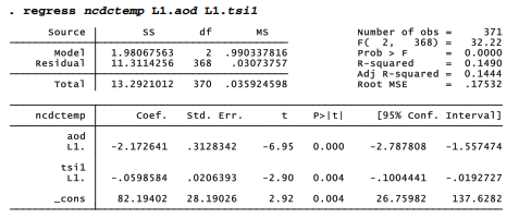
Adding a third predictor, lagged Multivariate ENSO Index, raises the explained variance further, R2a = .201. The coefficient on L1.mei is positive, as it should be given the known warming effect of El Nino. We still see an implausible negative coefficient on L1.tsil, however.
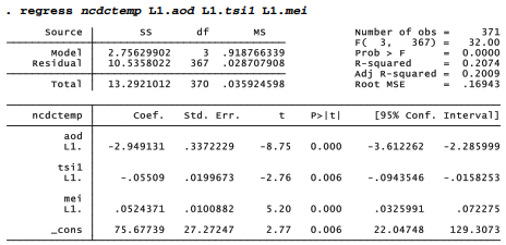
The most substantial improvement in R2a occurs when we include CO2 anomaly among the predictors. Together, these four drivers now explain 72.7% of the variance in monthly temperatures. CO2 anomaly has by far the strongest effect, in a positive direction as expected from the physics of greenhouse gases. Once we control for CO2, the coefficient on solar irradiance becomes positive as well.
. regress ncdctemp L1.aod L1.tsi1 L1.mei L1.co2anom
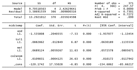
Figure 12.12 plots the progressive improvement of these four models. Predicted values in the lower right plot, based on the regression with all four drivers, track observed temperature remarkably well — including details such as the cooling after Pinatubo erupted, a warm spike during the “super El Niño” of 1998, and the wandering path of the past decade, cooled by low solar irradiance and low to negative ENSO. The fit between observed and predicted temperatures is striking also because the predictions come from an extremely simplified model in which all effects are linear, and operate with just one-month lags.
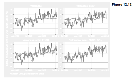
Global climate models based on physics instead of statistics, incorporating many more variables and vastly greater geographic complexity, may take weeks to run on a supercomputer. The appeal of the results graphed in Figure 12.12 is that such a simplified model performs as well
as it does, given its limitations. One of these limitations is statistical: OLS standard errors are biased, and the usual t and F tests invalid, if correlations occur among the errors. One simple check for correlated errors, called the Durbin-Watson test, can be run after any regression.
![]()
Statistical textbooks provide tables of critical values for the Durbin-Watson test. Given 5 estimated parameters (4 predictors and the y intercept) and 371 observations, these critical values are approximately dL = 1.59 and dv = 1.76. A test statistic below dL = 1.59 leads to rejecting the null hypothesis of no positive first-order (lag 1) autocorrelation. Because our calculated statistic, 1.131, is well below dL = 1.59, we should reject this null hypothesis and conclude instead that there does exist positive first-order autocorrelation. This finding confirms earlier suspicions about the validity of tests in our OLS models for temperature.
Had the calculated statistic been above dv = 1.76, we would fail to reject the null hypothesis. That is, we would then have no evidence of significant autocorrelation. Calculated Durbin-Watson statistics between dL and dv are inconclusive, neither rejecting nor failing to reject H0.
The Durbin-Watson statistic tests first-order autocorrelation, and ordinarily considers only the alternative hypothesis that it is positive. In practice, autocorrelation can be negative or positive, and can occur at other lags besides 1. The next section presents more general diagnostic tools.
Source: Hamilton Lawrence C. (2012), Statistics with STATA: Version 12, Cengage Learning; 8th edition.
23 Sep 2022
3 Oct 2022
3 Oct 2022
3 Oct 2022
28 Sep 2022
28 Sep 2022