Diagnosing Multicollinearity and Heteroskedasticity in Linear Regression by using Stata

Multicollinearity refers to the problem of too-strong linear relationships among the predictors or independent variables in a model. If perfect multicollinearity exists among the predictors, regression equations lack unique solutions. Stata warns us and then drops one of the offending predictors. High but not perfect multicollinearity causes more subtle problems. When we add a new predictor that is strongly related to predictors already in the model, symptoms of possible trouble include the following:

• Substantially higher standard errors, with correspondingly lower t
• Unexpected changes in coefficient magnitudes or signs.
• Nonsignificant coefficients despite a high R².

Multiple regression attempts to estimate the independent effects of each x variable. There is little information for doing so, however, if one or more of the x variables does not have much independent variation. The symptoms listed above warn that coefficient estimates have become unreliable, and might shift drastically with small changes in the data or model. Further troubleshooting is needed to determine whether multicollinearity really is at fault and, if so, what should be done about it.

Correlation matrices often are consulted as a diagnostic, but they have limited value for detecting multicollinearity. Correlations can only reveal collinearity, or linear relationships among variable pairs. Multicollinearity, on the other hand, involves linear relationships among any combination of independent variables, which might not be apparent from correlations. Better diagnostics are provided by the postestimation command estat vif, for variance inflation factor.

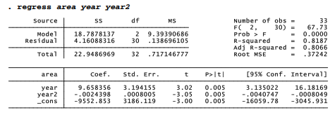
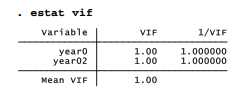
The 1/VIF column at right in an estat vif table gives values equal to 1 – R² from the regression of each x on the other x variables. Our Arctic ice example presents an extreme case: only .000005, less than .0005 percent, of the variance ofyear is independent ofyear2 (or vice versa). The variance inflation factor or VIF values themselves indicate that, with both predictors in the model, the variance of their coefficients is about 220,000 times higher than it otherwise would be. The standard error on year in the simple linear model seen earlier in this chapter is .0076648; the corresponding standard error in the quadratic model above is many times higher, 3.194155.

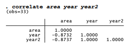
These VIF values indicate serious collinearity. Because there are only two predictors, in this instance we can confirm that observation just by looking at their correlations. year and year2 correlate almost perfectly.

Collinearity or multicollinearity can occur in any kind of model, but they are particularly common in models where some predictors are defined from others — such as those with interaction effects, or quadratic regression. The simple trick of centering, recommended earlier for interaction terms, can help with quadratic regression too. By reducing multicollinearity, centering often yields more precise coefficient estimates with lower standard errors.

We accomplish centering by subtracting the mean from one x variable before calculating the second. The mean year in these data is 1995; a centered version here called year0 represents years before 1995 (negative) or after 1995 (positive). Centered year0 has a mean of 0. A second new variable, year02, equals year0 squared. Its values range from 256 (when year0 = -16, meaning 1979) to 0 (when year0 = 0, meaning 1995), and then back up to 256 (when year0 = +16, meaning 2011).

After centering, differences will be most noticeable in the centered variable’s coefficient and standard error. To see this, we regress sea ice area on year0 and year02. The R² and overall F test are exactly as they were in the regression of area on uncentered year and year2. Predicted
values and residuals will be the same too. In the centered version, however, standard errors on yearO are much lower, confidence intervals narrower, t statistics larger, and t test results “more significant” than they were in the uncentered regression with plain year.

Although year and year2 correlate almost perfectly, centered versions have a correlation near 0.

Because the two predictors are uncorrelated, no variance inflation occurs.

The estat command obtains other useful diagnostic statistics as well. For example, estat hettest performs a heteroskedasticity test for the assumption of constant error variance. It does this by examining whether squared standardized residuals are linearly related to predicted values (see Cook and Weisberg 1994 for discussion and example). As seen below, estat hettest here gives no reason to reject the null hypothesis of constant variance. That is, we see no significant heteroskedasticity.

Presence of significant heteroskedasticity, on the other hand, would imply that our standard errors could be biased, and the resulting hypothesis tests invalid.

Source: Hamilton Lawrence C. (2012), Statistics with STATA: Version 12, Cengage Learning; 8th edition.