Repeated Measurements by using Stata

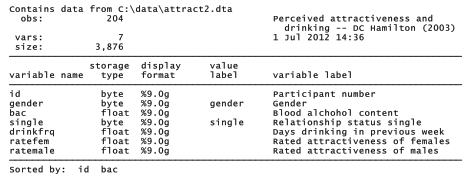
Dataset attract2.dta describes an unusual experiment carried out at a college undergraduate party, where some drinking apparently took place. In this experiment, 51 college students were asked to individually rate the attractiveness, on a scale from 1 to 10, of photographs of men and women unknown to them. The rating exercise was repeated by each participant, given the same photos shuffled in random order, on four occasions over the course of the evening. Variable ratemale is the mean rating each participant gave to all the male photos in one sitting, and ratefem is the mean rating given to female photos. gender records the subject’s own gender, and bac his or her blood alcohol content as measured by a breathalyzer.

. use C:\data\attract2.dta, clear

. describe

The research hypothesis involves a “beer goggles” effect: do strangers become more attractive as subjects consume more alcohol? In terms of this experiment, is there a positive relationship between blood alcohol content and the attractiveness ratings given to the photographs? If so, does that relationship vary with the gender of subject or photograph?

Although the data contain 204 observations, these represent only 51 individual participants. It seems reasonable that individual participants might differ in their tendency to give relatively high or low ratings, and in their reaction to alcohol. A mixed-effects model with random intercepts and slopes can accommodate these likely complications. This situation differs from the preceding election example in that individual random intercepts and slopes will not be substantively interesting, since they describe anonymous individuals. Rather, they are data or experimental-design features for which we need to adjust when testing the main hypotheses.

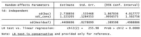
Using factor-variable notation, the following xtmixed command specifies a model in which mean ratings given to photographs of female faces (ratefem) are predicted by fixed effects of indicator variable gender, continuous variable bac, and their interaction. In addition, the model includes random intercepts and slopes for bac, which could vary across subjects.

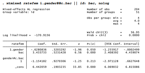
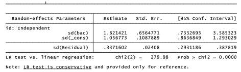
These results for female photographs support the beer goggles hypothesis: attractiveness ratings of female faces increase with blood alcohol content. Gender has a barely-significant effect: women gave slightly lower ratings to female faces. The gender^bac interaction is not significant. However, both the random intercept and the random slope on bac exhibit significant variation, indicating substantial person-to-person differences both in the mean ratings given, and in how alcohol affected those ratings.

margins and marginsplot commands help to visualize these results. Their outcome is not shown here, but will be combined with the next analysis to form Figure 13.8.

. margins, at(bac = (0(.2).4) gender = (0 1)) vsquish

. marginsplot, title(“Female photos”) ytitle(“”) xtitle(“”) noci

legend(position(11) ring(0) row(2)

title(“Gender”, size(medsmall)))

ylabel(4(1)8, grid gmin gmax)

plot1opts(lpattern(solid) msymbol(T))

plot2opts(lpattern(dash) msymbol(Oh)) saving(fig13_08RF)

A second xtmixed command models the ratings of male photographs (ratemal):

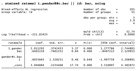
There does not seem to be a beer goggles effect on how male photographs are rated. On the other hand, gender exhibits a strong fixed effect. The interaction of gender and bac is not significant, but again we see significant variation in the random intercept and slope.

. margins, at(bac = (0(.2).4) gender = (0 1)) vsquish

. marginsplot, title(“Male photos”) ytitle(“”)

xtitle(“”) noci legend(position(11) ring(0) row(2)

title(“Gender”, size(medsmall))) ylabel(4(1)8, grid gmin gmax)

plot1opts(lpattern(solid) msymbol(T))

plot2opts(lpattern(dash) msymbol(Oh)) saving(fig13_08RM)

Figure 13.8 combines the two marginsplot graphs for direct comparison.

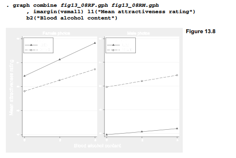
The left panel in Figure 13.8 visualizes the significant alcohol effect on ratings of female photographs. Male subjects gave somewhat higher ratings, and they appear slightly more affected by drink. The right panel depicts a different situation for ratings of male photographs.

Female subjects gave notably higher ratings, but neither male nor female subjects’ ratings changed much as they drank.

Source: Hamilton Lawrence C. (2012), Statistics with STATA: Version 12, Cengage Learning; 8th edition.