Describing Risks concerning consumer behavior

To describe risk quantitatively, we begin by listing all the possible outcomes of a particular action or event, as well as the likelihood that each outcome will occur.1  Suppose, for example, that you are considering investing in a company that explores for offshore oil. If the exploration effort is successful, the compa- ny’s stock will increase from $30 to $40 per share; if not, the price will fall to $20 per share. Thus there are two possible future outcomes: a $40-per-share price and a $20-per-share price.

1. Probability

Probability is the likelihood that a given outcome will occur. In our example, the probability that the oil exploration project will be successful might be 1/4 and the probability that it is unsuccessful 3/4.  (Note that the probabilities for all possible events must add up to 1.)

Our interpretation of probability can depend on the nature of the uncertain event, on the beliefs of the people involved, or both. One objective interpretation of probability relies on the frequency with which certain events tend to occur. Suppose we know that of the last 100 offshore oil explorations, 25 have suc- ceeded and 75 failed. In that case, the probability of success of 1/4  is objective because it is based directly on the frequency of similar experiences.

But what if there are no similar past experiences to help measure probabil- ity? In such instances, objective measures of probability cannot be deduced and more subjective measures are needed. Subjective probability is the perception that an outcome will occur. This perception may be based on a person’s judgment or experience, but not necessarily on the frequency with which a particular outcome has actually occurred in the past. When probabilities are subjectively determined, different people may attach different probabilities to different out- comes and thereby make different choices. For example, if the search for oil were to take place in an area where no previous searches had ever occurred, I might attach a higher subjective probability than you to the chance that the project will succeed: Perhaps I know more about the project or I have a better understand- ing of the oil business and can therefore make better use of our common infor- mation. Either different information or different abilities to process the same information can cause subjective probabilities to vary among individuals.

Regardless of the interpretation of probability, it is used in calculating two important measures that help us describe and compare risky choices. One mea- sure tells us the expected value and the other the variability of the possible outcomes.

2. Expected Value

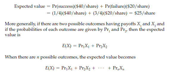
The expected value associated with an uncertain situation is a weighted aver- age of the payoffs or values associated with all possible outcomes. The prob- abilities of each outcome are used as weights. Thus the expected value measures the central tendency—the payoff or value that we would expect on average.

Our offshore oil exploration example had two possible outcomes: Success yields a payoff of $40 per share, failure a payoff of $20 per share. Denoting “probability of” by Pr, we express the expected value in this case as

3. Variability

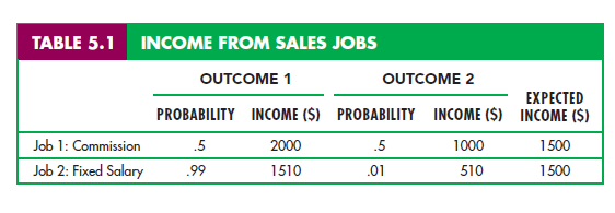
Variability is the extent to which the possible outcomes of an uncertain situation differ. To see why variability is important, suppose you are choosing between two part-time summer sales jobs that have the same expected income ($1500). The first job is based entirely on commission—the income earned depends on how much you sell. There are two equally likely payoffs for this job: $2000 for a successful sales effort and $1000 for one that is less successful. The second job is salaried. It is very likely (.99 probability) that you will earn $1510, but there is a .01 probability that the company will go out of business, in which case you would earn only $510 in severance pay. Table 5.1 summarizes these possible outcomes, their payoffs, and their probabilities.

Note that these two jobs have the same expected income. For Job 1, expected income is .5($2000) + .5($1000) = $1500; for Job 2, it is .99($1510) + .01($510) = $1500. However, the variability of the possible payoffs is different. We measure

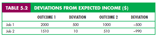
variability by recognizing that large differences between actual and expected pay- offs (whether positive or negative) imply greater risk. We call these differences deviations. Table 5.2 shows the deviations of the possible income from the expected income from each job.

By themselves, deviations do not provide a measure of variability. Why? Because they are sometimes positive and sometimes negative, and as you can see from Table 5.2, the average of the probability-weighted deviations is always 0.2

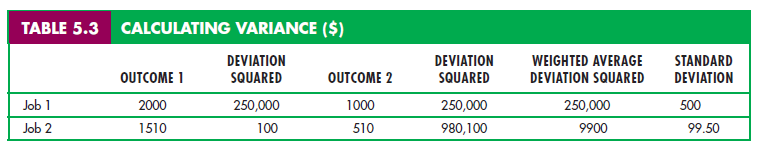
To get around this problem, we square each deviation, yielding numbers that are always positive. We then measure variability by calculating the standard deviation: the square root of the average of the squares of the deviations of the payoffs associated with each outcome from their expected values.3

Table 5.3 shows the calculation of the standard deviation for our example. Note that the average of the squared deviations under Job 1 is given by

.5($250,000) + .5($250,000) =  $250,000

The standard deviation is therefore equal to the square root of $250,000, or $500. Likewise, the probability-weighted average of the squared deviations under Job 2 is

.99($100) + .01($980,100) =  $9900

The standard deviation is the square root of $9900, or $99.50. Thus the second job is much less risky than the first; the standard deviation of the incomes is much lower.4

The concept of standard deviation applies equally well when there are many outcomes rather than just two. Suppose, for example, that the first summer job yields incomes ranging from $1000 to $2000 in increments of $100 that are all equally likely. The second job yields incomes from $1300 to $1700 (again in increments of $100) that are also equally likely. Figure 5.1 shows the alternatives graphically. (If there had been only two equally probable outcomes, then the figure would be drawn as two vertical lines, each with a height of 0.5.)

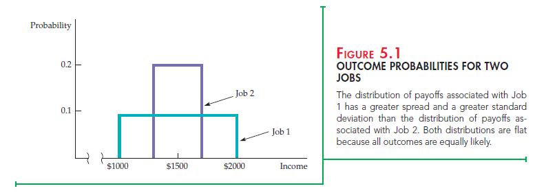
You can see from Figure 5.1 that the first job is riskier than the second. The “spread” of possible payoffs for the first job is much greater than the spread for the second. As a result, the standard deviation of the payoffs associated with the first job is greater than that associated with the second.

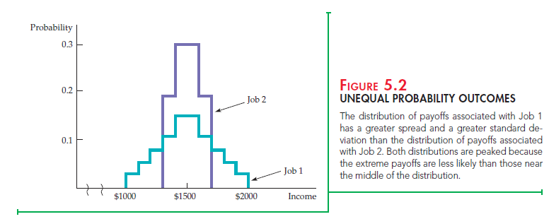
In this particular example, all payoffs are equally likely. Thus the curves describing the probabilities for each job are flat. In many cases, however, some payoffs are more likely than others. Figure 5.2 shows a situation in which the most extreme payoffs are the least likely. Again, the salary from Job 1 has a greater standard deviation. From this point on, we will use the standard deviation of payoffs to measure the degree of risk.

4. Decision Making

Suppose you are choosing between the two sales jobs described in our original example. Which job would you take? If you dislike risk, you will take the second job: It offers the same expected income as the first but with less risk. But suppose we add $100 to each of the payoffs in the first job, so that the expected payoff increases from $1500 to $1600. Table 5.4 gives the new earnings and the squared deviations.

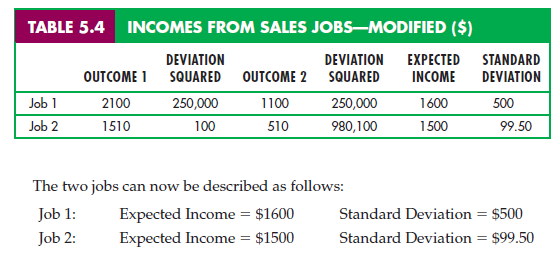
The two jobs can now be described as follows:

Job 1 offers a higher expected income but is much riskier than Job 2. Which job is preferred depends on the individual. While an aggressive entrepreneur who doesn’t mind taking risks might choose Job 1, with the higher expected income and higher standard deviation, a more conservative person might choose the second job.

People’s attitudes toward risk affect many of the decisions they make. In Example 5.1 we will see how attitudes toward risk affect people’s willingness to break the law, and how this has implications for the fines that should be set for various violations. Then in Section 5.2, we will further develop our theory of consumer choice by examining people’s risk preferences in greater detail.

Source: Pindyck Robert, Rubinfeld Daniel (2012), Microeconomics, Pearson, 8th edition.