This appendix presents a mathematical treatment of the basics of demand theory. Our goal is to provide a short overview of the theory of demand for students who have some familiarity with the use of calculus. To do this, we will explain and then apply the concept of constrained optimization.
1. Utility Maximization
The theory of consumer behavior is based on the assumption that consumers maximize utility subject to the constraint of a limited budget. We saw in Chapter 3 that for each consumer, we can define a utility function that attaches a level of util- ity to each market basket. We also saw that the marginal utility of a good is defined as the change in utility associated with a one-unit increase in the consumption of the good. Using calculus, as we do in this appendix, we measure marginal utility as the utility change that results from a very small increase in consumption.
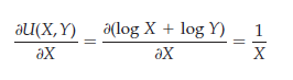
Suppose, for example, that Bob’s utility function is given by U(X, Y) = log X + log Y, where, for the sake of generality, X is now used to represent food and Y represents clothing. In that case, the marginal utility associated with the additional consumption of X is given by the partial derivative of the utility function with respect to good X. Here, MUX, representing the marginal utility of good X, is given by
In the following analysis, we will assume, as in Chapter 3, that while the level of utility is an increasing function of the quantities of goods consumed, marginal utility decreases with consumption. When there are two goods, X and Y, the consumer’s optimization problem may thus be written as
Maximize U(X, Y) (A4.1)
subject to the constraint that all income is spent on the two goods:
PXX + PyY = 1 (A4.2)
Here, U( ) is the utility function, X and Y the quantities of the two goods purchased, PX and PY the prices of the goods, and I income.[1]
To determine the individual consumer’s demand for the two goods, we choose those values of X and Y that maximize (A4.1) subject to (A4.2). When we know the particular form of the utility function, we can solve to find the consumer’s demand for X and Y directly. However, even if we write the utility function in its general form U(X, Y), the technique of constrained optimization can be used to describe the conditions that must hold if the consumer is maximizing utility.
2. The Method of Lagrange Multipliers
The method of Lagrange multipliers is a technique that can be used to max- imize or minimize a function subject to one or more constraints. Because we will use this technique to analyze production and cost issues later in the book, we will provide a step-by-step application of the method to the problem of finding the consumer ’s optimization given by equations (A4.1) and (A4.2).
The method of Lagrange multipliers is a technique that can be used to maximize or minimize a function subject to one or more constraints. Because we will use this technique to analyze production and cost issues later in the book, we will provide a step-by-step application of the method to the problem of finding the consumer’s optimization given by equations (A4.1) and (A4.2).
- Stating the Problem First, we write the Lagrangian for the problem. The Lagrangian is the function to be maximized or minimized (here, utility is being maximized), plus a variable which we call X times the constraint (here, the consumer’s budget constraint). We will interpret the meaning of X in a moment. The Lagrangian is then
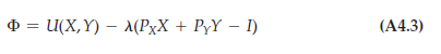
Note that we have written the budget constraint as
PXX + PyY – I = 0
i.e., as a sum of terms that is equal to zero. We then insert this sum into the Lagrangian.
- Differentiating the Lagrangian If we choose values of X and Y that satisfy the budget constraint, then the second term in equation (A4.3) will be zero. Maximizing will therefore be equivalent to maximizing U(X, Y). By differentiating $ with respect to X, Y, and X and then equating the derivatives to zero, we can obtain the necessary conditions for a maximum.[1] The resulting equations are
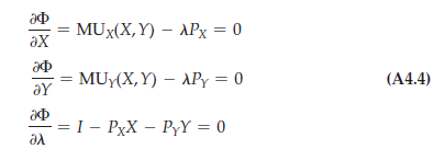
Here as before, MU is short for marginal utility: In other words, MUX(X, Y) = dU(X, Y)/dX, the change in utility from a very small increase in the consumption of good X.
- Solving the Resulting Equations The three equations in (A4.4) can be rewritten as
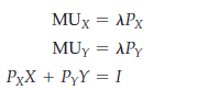
Now we can solve these three equations for the three unknowns. The resulting values of X and Y are the solution to the consumer ’s optimization problem: They are the utility-maximizing quantities.
3. The Equal Marginal Principle
The third equation above is the consumer’s budget constraint with which we started. The first two equations tell us that each good will be consumed up to the point at which the marginal utility from consumption is a multiple (X) of the price of the good. To see the implication of this, we combine the first two conditions to obtain the equal marginal principle:
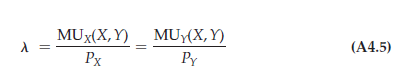
In other words, the marginal utility of each good divided by its price is the same. To optimize, the consumer must get the same utility from the last dollar spent by consuming either X or Y. If this were not the case, consuming more of one good and less of the other would increase utility.
To characterize the individual’s optimum in more detail, we can rewrite the information in (A4.5) to obtain
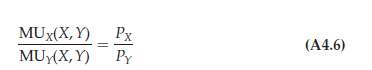
In other words, the ratio of the marginal utilities is equal to the ratio of the prices.
4. Marginal Rate of Substitution
We can use equation (A4.6) to see the link between utility functions and indifference curves that was spelled out in Chapter 3. An indifference curve represents all market baskets that give the consumer the same level of utility. If U* is a fixed utility level, the indifference curve that corresponds to that utility level is given by
U(X, Y) = U*
As the market baskets are changed by adding small amounts of X and subtracting small amounts of Y, the total change in utility must equal zero. Therefore,
MUx(X, Y)dX + MUy(X, Y)dY = dU* = 0
Rearranging,
– dY/dX = MUX(X, Y)/MUy(X, Y) = MRS XY (A4.8)
where MRSXY represents the individual’s marginal rate of substitution of X for Y. Because the left-hand side of (A4.8) represents the negative of the slope of the indifference curve, it follows that at the point of tangency, the individual’s marginal rate of substitution (which trades off goods while keeping utility constant) is equal to the individual’s ratio of marginal utilities, which in turn is equal to the ratio of the prices of the two goods, from (A4.6).[1]
When the individual indifference curves are convex, the tangency of the indifference curve to the budget line solves the consumer’s optimization problem. This principle was illustrated by Figure 3.13 (page 86) in Chapter 3.
[1]We implicitly assume that the “second-order conditions” for a utility maximum hold. The consumer, therefore, is maximizing rather than minimizing utility. The convexity condition is sufficient for the second-order conditions to be satisfied. In mathematical terms, the condition is that d(MRS)/dX < 0 or that dY2/dX2 > 0 where — dY/dX is the slope of the indifference curve. Remember: diminishing marginal utility is not sufficient to ensure that indifference curves are convex.
5. Marginal Utility of Income
Whatever the form of the utility function, the Lagrange multiplier X represents the extra utility generated when the budget constraint is relaxed—in this case by adding one dollar to the budget. To show how the principle works, we differentiate the utility function U(X, Y) totally with respect to I:
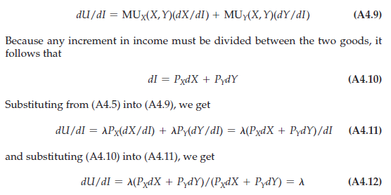
Thus the Lagrange multiplier is the extra utility that results from an extra dollar of income.
Going back to our original analysis of the conditions for utility maximization, we see from equation (A4.5) that maximization requires the utility obtained from the consumption of every good, per dollar spent on that good, to be equal to the marginal utility of an additional dollar of income. If this were not the case, utility could be increased by spending more on the good with the higher ratio of marginal utility to price and less on the other good.
6. An Example
In general, the three equations in (A4.4) can be solved to determine the three unknowns X, Y, and X as a function of the two prices and income. Substitution for X then allows us to solve for the demand for each of the two goods in terms of income and the prices of the two commodities. This principle can be most easily seen in terms of an example.
A frequently used utility function is the Cobb-Douglas utility function,
which can be represented in two forms:
U(X, Y) = a log(X) + (1 – a) log(Y)
and
U(X, Y) = XaY1 – a
For the purposes of demand theory, these two forms are equivalent because they both yield the identical demand functions for goods X and Y. We will derive the demand functions for the first form and leave the second as an exercise for the student.
To find the demand functions for X and Y, given the usual budget constraint, we first write the Lagrangian:
![]()
Now differentiating with respect to X, Y, and X and setting the derivatives equal to zero, we obtain
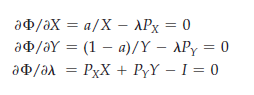
The first two conditions imply that
Combining these expressions with the last condition (the budget constraint)
gives us
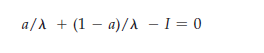
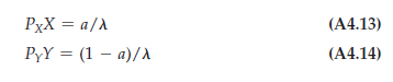
or X = 1/I. Now we can substitute this expression for X back into (A4.13) and (A4.14) to obtain the demand functions:
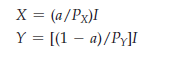
In this example, the demand for each good depends only on the price of that good and on income, not on the price of the other good. Thus, the cross-price elasticities of demand are 0.
We can also use this example to review the meaning of Lagrange multipliers. To do so, let’s substitute specific values for each of the parameters in the problem. Let a = 1/2, PX = $1, PY = $2, and I = $100. In this case, the choices that maximize utility are X = 50 and Y = 25. Also note that X = 1/100. The Lagrange multiplier tells us that if an additional dollar of income were available to the consumer, the level of utility achieved would increase by 1/100. This conclusion is relatively easy to check. With an income of $101, the maximizing choices of the two goods are X = 50.5 and Y = 25.25. A bit of arithmetic tells us that the original level of utility is 3.565 and the new level of utility 3.575. As we can see, the additional dollar of income has indeed increased utility by .01, or 1/100.
7. Duality in Consumer Theory
There are two different ways of looking at the consumer ’s optimization deci- sion. The optimum choice of X and Y can be analyzed not only as the problem of choosing the highest indifference curve—the maximum value of U( )—that touches the budget line, but also as the problem of choosing the lowest budget line—the minimum budget expenditure—that touches a given indifference curve. We use the term duality to refer to these two perspectives. To see how this principle works, consider the following dual consumer optimization problem: the problem of minimizing the cost of achieving a particular level of utility:
Minimize PXX + PyY
subject to the constraint that
U(X, Y) = U*
The corresponding Lagrangian is given by
![]()
where p is the Lagrange multiplier. Differentiating $ with respect to X, Y, and p and setting the derivatives equal to zero, we find the following necessary conditions for expenditure minimization:
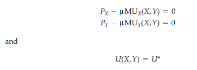
By solving the first two equations, and recalling (A4.5), we see that p = [Px/MUx(X, Y)] = [Py/MUy(X, Y)] = 1/1 Because it is also true that
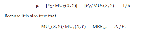
the cost-minimizing choice of X and Y must occur at the point of tangency of the budget line and the indifference curve that generates utility U*. Because this is the same point that maximized utility in our original problem, the dual expenditure- minimization problem yields the same demand functions that are obtained from the direct utility-maximization problem.
To see how the dual approach works, let’s reconsider our Cobb-Douglas example. The algebra is somewhat easier to follow if we use the exponential form of the Cobb-Douglas utility function, U(X, Y) = XY – a. In this case, the Lagrangian is given by
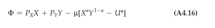
Differentiating with respect to X, Y, and p and equating to zero, we obtain
Multiplying the first equation by X and the second by Y and adding, we get
![]()
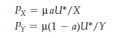
First, we let I be the cost-minimizing expenditure (if the individual did not spend all of his income to get utility level U*, U* would not have maximized utility in the original problem). Then it follows that p = I/U*. Substituting in the equations above, we obtain
![]()
These are the same demand functions that we obtained before.
8. Income and Substitution Effects
The demand function tells us how any individual’s utility-maximizing choices respond to changes in both income and the prices of goods. It is important, how- ever, to distinguish that portion of any price change that involves movement along an indifference curve from that portion which involves movement to a different indiffer- ence curve (and therefore a change in purchasing power). To make this distinction, we consider what happens to the demand for good X when the price of X changes. As we explained in Section 4.2, the change in demand can be divided into a sub- stitution effect (the change in quantity demanded when the level of utility is fixed) and an income effect (the change in the quantity demanded with the level of utility changing but the relative price of good X unchanged). We denote the change in X that results from a unit change in the price of X, holding utility constant, by
![]()
Thus the total change in the quantity demanded of X resulting from a unit change in PX is
![]()
The first term on the right side of equation (A4.17) is the substitution effect (because utility is fixed); the second term is the income effect (because income increases).
From the consumer’s budget constraint, I = PXX + PyY, we know by differentiation that
![]()
Suppose for the moment that the consumer owned goods X and Y. In that case, equation (A4.18) would tell us that when the price of good X increases by $1, the amount of income that the consumer can obtain by selling the good increases by $X. In our theory of consumer behavior, however, the consumer does not own the good. As a result, equation (A4.18) tells us how much additional income the consumer would need in order to be as well off after the price change as he or she was before. For this reason, it is customary to write the income effect as negative (reflecting a loss of purchasing power) rather than as a positive. Equation (A4.17) then appears as follows:
![]()
In this new form, called the Slutsky equation, the first term represents the substitution effect: the change in demand for good X obtained by keeping utility fixed. The second term is the income effect: the change in purchasing power resulting from the price change times the change in demand resulting from a change in purchasing power.
An alternative way to decompose a price change into sustitution and income effects, which is usually attributed to John Hicks, does not involve indifference curves. In Figure A4.1, the consumer initially chooses market basket A on budget line RS. Suppose that after the price of food falls (and the budget line moves to RT), we take away enough income so that the individual is no better off (and no worse off) than he was before. To do so, we draw a budget line parallel to RT. If the budget line passed through A, the consumer would be at least as satisfied as he was before the price change: He still has the option to purchase market basket A if he wishes. According to the Hicksian substitution effect, therefore, the budget line that leaves him equally well off must be a line such as R’T’, which is parallel to RT and which intersects RS at a point B below and to the right of point A.
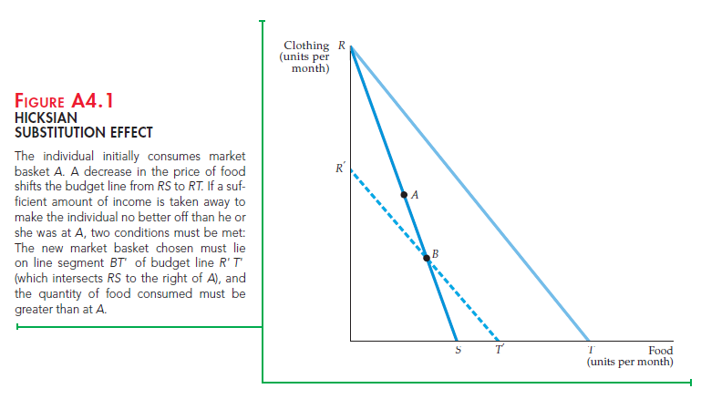
Revealed preference tells us that the newly chosen market basket must lie on line segment BT‘. Why? Because all market baskets on line segment R‘ B could have been chosen but were not when the original budget line was RS. (Recall that the consumer preferred basket A to any other feasible market basket.) Now note that all points on line segment BT‘ involve more food consumption than does basket A. It follows that the quantity of food demanded increases whenever there is a decrease in the price of food with utility held constant. This negative substitution effect holds for all price changes and does not rely on the assumption of convexity of indifference curves that we made in Section 3.1 (page 69).
Source: Pindyck Robert, Rubinfeld Daniel (2012), Microeconomics, Pearson, 8th edition.
Hello my friend! I wish to say that this article is amazing, great written and include almost all significant infos. I would like to peer extra posts like this .