We used a job example to show how people might evaluate risky outcomes, but the principles apply equally well to other choices. In this section, we concentrate on consumer choices generally and on the utility that consumers obtain from choosing among risky alternatives. To simplify things, we’ll consider the util- ity that a consumer gets from his or her income—or, more appropriately, the market basket that the consumer ’s income can buy. We now measure payoffs, therefore, in terms of utility rather than dollars.
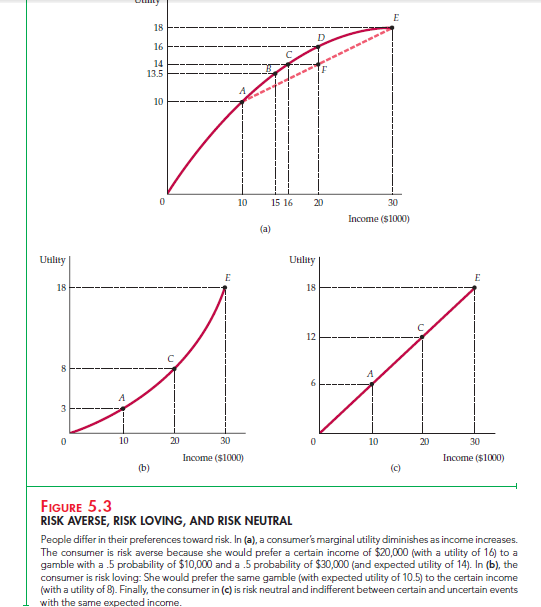
Figure 5.3 (a) shows how we can describe one woman’s preferences toward risk. The curve 0E, which gives her utility function, tells us the level of utility (on the vertical axis) that she can attain for each level of income (measured in thousands of dollars on the horizontal axis). The level of utility increases from
10 to 16 to 18 as income increases from $10,000 to $20,000 to $30,000. But note that marginal utility is diminishing, falling from 10 when income increases from
0 to $10,000, to 6 when income increases from $10,000 to $20,000, and to 2 when income increases from $20,000 to $30,000.
Now suppose that our consumer has an income of $15,000 and is considering a new but risky sales job that will either double her income to $30,000 or cause it to fall to $10,000. Each possibility has a probability of .5. As Figure 5.3 (a) shows, the utility level associated with an income of $10,000 is 10 (at point A) and the utility level associated with an income of $30,000 is 18 (at E). The risky job must be compared with the current $15,000 job, for which the utility is 13.5 (at B).
To evaluate the new job, she can calculate the expected value of the resulting income. Because we are measuring value in terms of her utility, we must calcu- late the expected utility E(u) that she can obtain. The expected utility is the sum of the utilities associated with all possible outcomes, weighted by the probability that each outcome will occur. In this case expected utility is
E(u) = (1/2)u($10,000) + (1/2)u($30,000) = 0.5(10) + 0.5(18) = 14
The risky new job is thus preferred to the original job because the expected utility of 14 is greater than the original utility of 13.5.
The old job involved no risk—it guaranteed an income of $15,000 and a util- ity level of 13.5. The new job is risky but offers both a higher expected income ($20,000) and, more importantly, a higher expected utility. If the woman wishes to increase her expected utility, she will take the risky job.
1. Different Preferences Toward Risk
People differ in their willingness to bear risk. Some are risk averse, some risk loving, and some risk neutral. An individual who is risk averse prefers a cer- tain given income to a risky income with the same expected value. (Such a per- son has a diminishing marginal utility of income.) Risk aversion is the most common attitude toward risk. To see that most people are risk averse most of the time, note that most people not only buy life insurance, health insurance, and car insurance, but also seek occupations with relatively stable wages.
Figure 5.3 (a) applies to a woman who is risk averse. Suppose hypothetically that she can have either a certain income of $20,000, or a job yielding an income of $30,000 with probability .5 and an income of $10,000 with probability .5 (so that the expected income is also $20,000). As we saw, the expected utility of the uncertain income is 14—an average of the utility at point A(10) and the utility at E(18)—and is shown by F. Now we can compare the expected utility associated with the risky job to the utility generated if $20,000 were earned without risk. This latter utility level, 16, is given by D in Figure 5.3 (a). It is clearly greater than the expected utility of 14 associated with the risky job.
For a risk-averse person, losses are more important (in terms of the change in utility) than gains. Again, this can be seen from Figure 5.3 (a). A $10,000 increase in income, from $20,000 to $30,000, generates an increase in utility of two units; a $10,000 decrease in income, from $20,000 to $10,000, creates a loss of utility of six units.
A person who is risk neutral is indifferent between a certain income and an uncertain income with the same expected value. In Figure 5.3 (c) the utility associated with a job generating an income of either $10,000 or $30,000 with equal probability is 12, as is the utility of receiving a certain income of $20,000. As you can see from the figure, the marginal utility of income is constant for a risk-neutral person.6
Finally, an individual who is risk loving prefers an uncertain income to a certain one, even if the expected value of the uncertain income is less than that of the certain income. Figure 5.3 (b) shows this third possibility. In this case, the expected utility of an uncertain income, which will be either $10,000 with prob- ability .5 or $30,000 with probability .5, is higher than the utility associated with a certain income of $20,000. Numerically,
E(u) = .5u($10,000) + .5u($30,000) = .5(3) + .5(18) = 10.5 7 u($20,000) = 8
Of course, some people may be averse to some risks and act like risk lovers with respect to others. For example, many people purchase life insurance and are conservative with respect to their choice of jobs, but still enjoy gambling. Some criminologists might describe criminals as risk lovers, especially if they com- mit crimes despite a high prospect of apprehension and punishment. Except for such special cases, however, few people are risk loving, at least with respect to major purchases or large amounts of income or wealth.
RISK PREMIUM The risk premium is the maximum amount of money that a risk-averse person will pay to avoid taking a risk. In general, the magnitude of the risk premium depends on the risky alternatives that the person faces. To determine the risk premium, we have reproduced the utility function of Figure 5.3 (a) in Figure 5.4 and extended it to an income of $40,000. Recall that an expected utility of 14 is achieved by a woman who is going to take a risky job with an expected income of $20,000. This outcome is shown graphically by drawing a horizontal line to the vertical axis from point F, which bisects straight
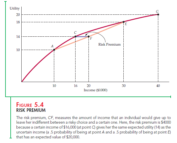
line AE (thus representing an average of $10,000 and $30,000). But the utility level of 14 can also be achieved if the woman has a certain income of $16,000, as shown by dropping a vertical line from point C. Thus, the risk premium of $4000, given by line segment CF, is the amount of expected income ($20,000 minus
$16,000) that she would give up in order to remain indifferent between the risky job and a hypothetical job that would pay her a certain income of $16,000.
RISK AVERSION AND INCOME The extent of an individual’s risk aversion depends on the nature of the risk and on the person’s income. Other things being equal, risk-averse people prefer a smaller variability of outcomes. We saw that when there are two outcomes—an income of $10,000 and an income of $30,000—the risk premium is $4000. Now consider a second risky job, also illustrated in Figure 5.4. With this job, there is a .5 probability of receiving an income of $40,000, with a util- ity level of 20, and a .5 probability of getting an income of $0, with a utility level of 0. The expected income is again $20,000, but the expected utility is only 10:
Expected utility = .5u($0) + .5u($40,000) = 0 + .5(20) = 10
Compared to a hypothetical job that pays $20,000 with certainty, the person holding this risky job gets 6 fewer units of expected utility: 10 rather than 16 units. At the same time, however, this person could also get 10 units of utility from a job that pays $10,000 with certainty. Thus the risk premium in this case is $10,000, because this person would be willing to give up $10,000 of her $20,000 expected income to avoid bearing the risk of an uncertain income. The greater the variability of income, the more the person would be willing to pay to avoid the risky situation.
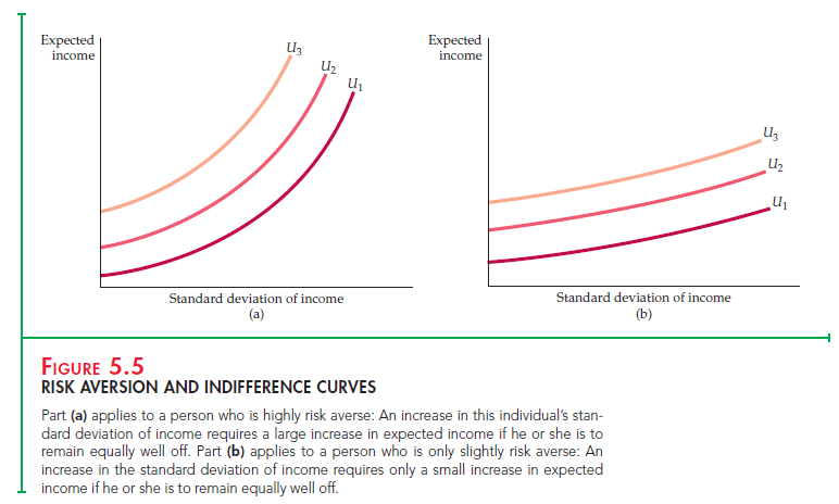
RISK AVERSION AND INDIFFERENCE CURVES We can also describe the extent of a person’s risk aversion in terms of indifference curves that relate expected income to the variability of income, where the latter is measured by the standard deviation. Figure 5.5 shows such indifference curves for two indi- viduals, one who is highly risk averse and another who is only slightly risk averse. Each indifference curve shows the combinations of expected income and standard deviation of income that give the individual the same amount of utility. Observe that all of the indifference curves are upward sloping: Because risk is undesirable, the greater the amount of risk, the greater the expected income needed to make the individual equally well off.
Figure 5.5 (a) describes an individual who is highly risk averse. Observe that in order to leave this person equally well off, an increase in the standard devia- tion of income requires a large increase in expected income. Figure 5.5 (b) applies to a slightly risk-averse person. In this case, a large increase in the standard deviation of income requires only a small increase in expected income.
Source: Pindyck Robert, Rubinfeld Daniel (2012), Microeconomics, Pearson, 8th edition.
Hello my family member! I wish to say that this post is awesome, great written and include approximately all vital infos. I’d like to look more posts like this .
Dude these articles have been really helpful to me. They really helped me out.
Thanks for your help and for writing this post. It’s been great.
Dude these articles were really helpful to me. Thanks a lot.
Thanks for the help
There is no doubt that your post was a big help to me. I really enjoyed reading it.
Thank you for your post. I really enjoyed reading it, especially because it addressed my issue. It helped me a lot and I hope it will also help others.
I truly appreciate this post. I?ve been looking everywhere for this! Thank goodness I found it on Bing. You’ve made my day! Thanks again