Industry’s Long-Run Supply Curve

In our analysis of short-run supply, we first derived the firm’s supply curve and then showed how the summation of individual firms’ supply curves gener- ated a market supply curve. We cannot, however, analyze long-run supply in the same way: In the long run, firms enter and exit markets as the market price changes. This makes it impossible to sum up supply curves—we do not know which firms’ supplies to add up in order to get market totals.

The shape of the long-run supply curve depends on the extent to which increases and decreases in industry output affect the prices that firms must pay for inputs into the production process. In cases in which there are economies of scale in production or cost savings associated with the purchase of large vol- umes of inputs, input prices will decline as output increases. In cases where diseconomies of scale are present, input prices may increase with output. The third possibility is that input costs may not change with output. In any of these cases, to determine long-run supply, we assume that all firms have access to the available production technology. Output is increased by using more inputs, not by invention. We also assume that the conditions underlying the market for inputs to production do not change when the industry expands or contracts. For example, an increased demand for labor does not increase a union’s ability to negotiate a better wage contract for its workers.

In our analysis of long-run supply, it will be useful to distinguish among three types of industries: constant cost, increasing cost, and decreasing cost.

1. Constant–Cost Industry

Figure 8.16 shows the derivation of the long-run supply curve for a constant- cost industry. A firm’s output choice is given in (a), while industry output is shown in (b). Assume that the industry is initially in equilibrium at the intersec- tion of market demand curve D1  and short-run market supply curve S1. Point A at the intersection of demand and supply is on the long-run supply curve SL because it tells us that the industry will produce Q1  units of output when the long-run equilibrium price is P1.

To obtain other points on the long-run supply curve, suppose the market demand for the product unexpectedly increases (say, because of a reduction in personal income taxes). A typical firm is initially producing at an output of q1, where P1 is equal to long-run marginal cost and long-run average cost. But because the firm is also in short-run equilibrium, price also equals short-run marginal cost.

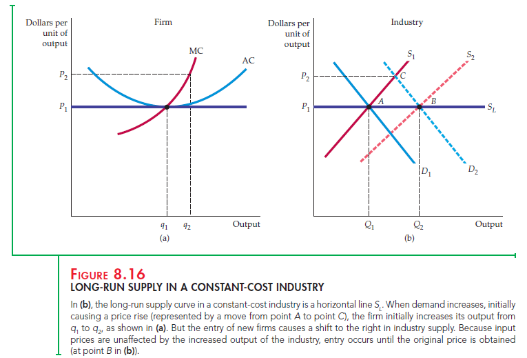
Suppose that the tax cut shifts the market demand curve from D1  to D2. Demand curve D2 intersects supply curve S1 at C. As a result, price increases from P1 to P2.

Part (a) of Figure 8.16 shows how this price increase affects a typical firm

in the industry. When the price increases to P2, the firm follows its short-run marginal cost curve and increases output to q2. This output choice maximizes profit because it satisfies the condition that price equal short-run marginal cost. If every firm responds this way, each will be earning a positive profit in short- run equilibrium. This profit will be attractive to investors and will cause exist- ing firms to expand operations and new firms to enter the market.

As a result, in Figure 8.16 (b) the short-run supply curve shifts to the right from S1  to S2. This shift causes the market to move to a new long-run equilib- rium at the intersection of D2  and S2. For this intersection to be a long-run equi- librium, output must expand enough so that firms are earning zero profit and the incentive to enter or exit the industry disappears.

In a constant-cost industry, the additional inputs necessary to produce higher output can be purchased without an increase in per-unit price. This might happen, for example, if unskilled labor is a major input in production, and the market wage of unskilled labor is unaffected by the increase in the demand for labor. Because the prices of inputs have not changed, firms’ cost curves are also unchanged; the new equilibrium must be at a point such as B in Figure 8.16 (b), at which price is equal to P1, the original price before the unexpected increase in demand occurred.

The long-run supply curve for a constant-cost industry is, therefore, a horizontal line at a price that is equal to the long-run minimum average cost of production. At any higher price, there would be positive profit, increased entry, increased short-run supply, and thus downward pressure on price. Remember that in a constant-cost industry, input prices do not change when conditions change in the output mar- ket. Constant-cost industries can have horizontal long-run average cost curves.

2. Increasing–Cost  Industry

In an increasing-cost industry the prices of some or all inputs to produc- tion increase as the industry expands and the demand for the inputs grows. Diseconomies of scale in the production of one or more inputs may be the explanation. Suppose, for example, that the industry uses skilled labor, which becomes in short supply as the demand for it increases. Or, if a firm requires mineral resources that are available only on certain types of land, the cost of land as an input increases with output. Figure 8.17 shows the derivation of long- run supply, which is similar to the previous constant-cost derivation. The indus- try is initially in equilibrium at A in part (b). When the demand curve unexpect- edly shifts from D1 to D2, the price of the product increases in the short run to P2, and industry output increases from Q1 to Q2. A typical firm, as shown in part (a), increases its output from q1 to q2 in response to the higher price by moving along its short-run marginal cost curve. The higher profit earned by this and other

firms induces new firms to enter the industry.

As new firms enter and output expands, increased demand for inputs causes some or all input prices to increase. The short-run market supply curve shifts to the right as before, though not as much, and the new equilibrium at B results in a price P3  that is higher than the initial price P1. Because the higher input prices raise the firms’ short-run and long-run cost curves, the higher market price is needed to ensure that firms earn zero profit in long-run equi- librium. Figure 8.17 (a) illustrates this. The average cost curve shifts up from AC1  to AC2, while the marginal cost curve shifts to the left, from MC1  to MC2. The new long-run equilibrium price P3  is equal to the new minimum average

cost. As in the constant-cost case, the higher short-run profit caused by the initial increase in demand disappears in the long run as firms increase output and input costs rise.

The new equilibrium at B in Figure 8.17 (b) is, therefore, on the long-run sup- ply curve for the industry. In an increasing-cost industry, the long-run industry supply curve is upward sloping. The industry produces more output, but only at the higher price needed to compensate for the increase in input costs. The term “increasing cost” refers to the upward shift in the firms’ long-run average cost curves, not to the positive slope of the cost curve itself.

3. Decreasing–Cost  Industry

The industry supply curve can also be downward sloping. In this case, the unexpected increase in demand causes industry output to expand as before. But as the industry grows larger, it can take advantage of its size to obtain some of its inputs more cheaply. For example, a larger industry may allow for an improved transportation system or for a better, less expensive financial net- work. In this case, firms’ average cost curves shift downward (even if they do not enjoy economies of scale), and the market price of the product falls. The lower market price and lower average cost of production induce a new long- run equilibrium with more firms, more output, and a lower price. Therefore, in a decreasing-cost industry, the long-run supply curve for the industry is downward sloping.

Source: Pindyck Robert, Rubinfeld Daniel (2012), Microeconomics, Pearson, 8th edition.