Inferences About the Difference Between Two Population Proportions

Letting p₁ denote the proportion for population 1 and p₂ denote the proportion for population 2, we next consider inferences about the difference between the two population proportions: P₁ – P₂. To make an inference about this difference, we will select two independent random samples consisting of n₁ units from population 1 and n₂ units from population 2.

1. Interval Estimation of p₁ — p₂

In the following example, we show how to compute a margin of error and develop an inter­val estimate of the difference between two population proportions.

A tax preparation firm is interested in comparing the quality of work at two of its regional offices. By randomly selecting samples of tax returns prepared at each office and verifying the sample returns’ accuracy, the firm will be able to estimate the proportion of erroneous returns prepared at each office. Of particular interest is the difference between these proportions.

The difference between the two population proportions is given by p₁ – p₂. The point estimator of p₁ – p₂ is as follows.

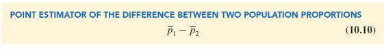
Thus, the point estimator of the difference between two population proportions is the dif­ference between the sample proportions of two independent simple random samples.

As with other point estimators, the point estimator p₁ – p₂ has a sampling distribution that reflects the possible values of p₁ – p₂ if we repeatedly took two independent random samples. The mean of this sampling distribution is p₁ – p₂ and the standard error of p₁ – p₂ is as follows:

If the sample sizes are large enough that n1p1, n1(1 − p1), n2p2, and n2(1 − p2) are all greater than or equal to 5, the sampling distribution of p₁ – p₂ can be approximated by a normal distribution.

As we showed previously, an interval estimate is given by a point estimate ± a margin of error. In the estimation of the difference between two population proportions, an interval estimate will take the following form:

p1 – p2 ± Margin of error

With the sampling distribution of p₁ — p₂ approximated by a normal distribution, we would like to use z_a/2&p_i _p as the margin of error. However, sp_i _p given by equation (10.11) cannot be used directly because the two population proportions, p₁ and p₂, are unknown. Using the sample proportion p₁ to estimate p₁ and the sample proportion p₂ to estimate p₂, the margin of error is as follows.

The general form of an interval estimate of the difference between two population propor­tions is as follows.

Returning to the tax preparation example, we find that independent simple random samples from the two offices provide the following information.

The sample proportions for the two offices follow.

The point estimate of the difference between the proportions of erroneous tax returns for the two populations is p₁ — p₂ = .14 — .09 = .05. Thus, we estimate that office 1 has a .05, or 5%, greater error rate than office 2.

Expression (10.13) can now be used to provide a margin of error and interval estimate of the difference between the two population proportions. Using a 90% confidence interval with z_a/2 = z.₀₅ = 1.645, we have

Thus, the margin of error is .045, and the 90% confidence interval is .005 to .095.

2. Hypothesis Tests About p₁ — p₂

Let us now consider hypothesis tests about the difference between the proportions of two populations. We focus on tests involving no difference between the two population propor­tions. In this case, the three forms for a hypothesis test are as follows:

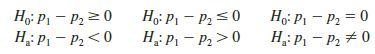
When we assume H₀ is true as an equality, we have P_i – p₂ = 0, which is the same as saying that the population proportions are equal, p_i = p₂.

We will base the test statistic on the sampling distribution of the point estimator p_i – p₂. In equation (i0.ii), we showed that the standard error of p_i – p₂ is given by

Under the assumption H₀ is true as an equality, the population proportions are equal and p_i = p₂ = p. In this case, σp1-p2 becomes

With p unknown, we pool, or combine, the point estimators from the two samples (p_i and p₂) to obtain a single point estimator of P as follows:

This pooled estimator of p is a weighted average of p_i and p₂.

Substituting p forp in equation (i0.i4), we obtain an estimate of the standard error of P_i – P₂. This estimate of the standard error is used in the test statistic. The general form of the test statistic for hypothesis tests about the difference between two population propor­tions is the point estimator divided by the estimate of σp1-p2

This test statistic applies to large sample situations where n₁p₁, n₁(1 – p₁), n₂p₂, and n₂(1 – p₂) are all greater than or equal to 5.

Let us return to the tax preparation firm example and assume that the firm wants to use a hypothesis test to determine whether the error proportions differ between the two offices. A two-tailed test is required. The null and alternative hypotheses are as follows:

If H₀ is rejected, the firm can conclude that the error rates at the two offices differ. We will use a = .10 as the level of significance.

The sample data previously collected showed p₁ = .14 for the n₁ = 250 returns sam­pled at office 1 and p₂ = .09 for the n₂ = 300 returns sampled at office 2. We continue by computing the pooled estimate of p.

Using this pooled estimate and the difference between the sample proportions, the value of the test statistic is as follows.

In computing the p-value for this two-tailed test, we first note that z = 1.85 is in the upper tail of the standard normal distribution. Using z = 1.85 and the standard normal distribution table, we find the area in the upper tail is 1.0000 – .9678 = .0322. Doubling this area for a two-tailed test, we find the p-value = 2(.0322) = .0644. With the p-value less than a = .10, H₀ is rejected at the .10 level of significance. The firm can conclude that the error rates dif­fer between the two offices. This hypothesis testing conclusion is consistent with the earlier interval estimation results that showed the interval estimate of the difference between the population error rates at the two offices to be .005 to .095, with Office 1 having the higher error rate.

Source:  Anderson David R., Sweeney Dennis J., Williams Thomas A. (2019), Statistics for Business & Economics, Cengage Learning; 14th edition.