In this section we show how to conduct significance tests for a multiple regression relationship. The significance tests we used in simple linear regression were a t test and an F test. In simple linear regression, both tests provide the same conclusion; that is, if the null hypothesis is rejected, we conclude that b1 A 0. In multiple regression, the t test and the F test have different purposes.
- The F test is used to determine whether a significant relationship exists between the dependent variable and the set of all the independent variables; we will refer to the F test as the test for overall significance.
- If the F test shows an overall significance, the t test is used to determine whether each of the individual independent variables is significant. A separate t test is conducted for each of the independent variables in the model; we refer to each of these t tests as a test for individual significance.
In the material that follows, we will explain the F test and the t test and apply each to the Butler Trucking Company example.
1. F Test
The multiple regression model as defined in Section 15.4 is
![]()
The hypotheses for the F test involve the parameters of the multiple regression model.
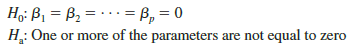
If H0 is rejected, the test gives us sufficient statistical evidence to conclude that one or more of the parameters are not equal to zero and that the overall relationship between y and the set of independent variables x1, x2, . . . , xp is significant. However, if H0 cannot be rejected, we do not have sufficient evidence to conclude that a significant relationship is present.
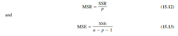
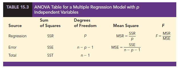
Before describing the steps of the F test, we need to review the concept of mean square. A mean square is a sum of squares divided by its corresponding degrees of freedom. In the multiple regression case, the total sum of squares has n – 1 degrees of freedom, the sum of squares due to regression (SSR) has p degrees of freedom, and the sum of squares due to error has n – p – 1 degrees of freedom. Hence, the mean square due to regression (MSR) is SSR/p and the mean square due to error (MSE) is SSE/(n – p – 1).
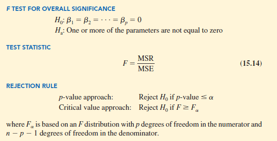
As discussed in Chapter 14, MSE provides an unbiased estimate of s2, the variance of the error term e. If H0: β1 = β2 = . . . = βp = 0 is true, MSR also provides an unbiased estimate of s2, and the value of MSR/MSE should be close to 1. However, if H0 is false, MSR overestimates s2 and the value of MSR/MSE becomes larger. To determine how large the value of MSR/MSE must be to reject H0, we make use of the fact that if H0 is true and the assumptions about the multiple regression model are valid, the sampling distribution of MSR/MSE is an F distribution with p degrees of freedom in the numerator and n – p – 1 in the denominator. A summary of the F test for significance in multiple regression follows.
Let us apply the F test to the Butler Trucking Company multiple regression problem. With two independent variables, the hypotheses are written as follows:
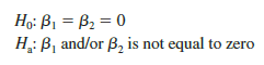
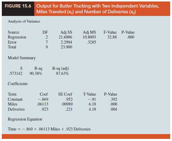
Figure 15.6 is the output for the multiple regression model with miles traveled (x1) and number of deliveries (x2) as the two independent variables. In the analysis of variance part of the output, we see that MSR = 10.8003 and MSE = .3285. Using equation (15.14), we obtain the test statistic.
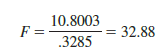
Using a = .01, the p-value = .000 in the last column of the analysis of variance table (Figure 15.6) indicates that we can reject H0: β1 = β2 = 0 because the p-value is less than a = .01. Alternatively, Table 4 of Appendix B shows that with two degrees of freedom in the numerator and seven degrees of freedom in the denominator, F.01 = 9.55. With 32.88 > 9.55, we reject H0: β1 = β2 = 0 and conclude that a significant relationship is present between travel time y and the two independent variables, miles traveled and number of deliveries.
As noted previously, the mean square error provides an unbiased estimate of a2, the variance of the error term e. Referring to Figure 15.6, we see that the estimate of a2 is MSE = .3285. The square root of MSE is the estimate of the standard deviation of the error term. As defined in Section 14.5, this standard deviation is called the standard error of the estimate and is denoted 5. Hence, we have 5 = √MSE = √.3285 = .5731. Note that the value of the standard error of the estimate appears in the output in Figure 15.6.
Table 15.3 is the general analysis of variance (ANOVA) table that provides the F test results for a multiple regression model. The value of the F test statistic appears in the last column and can be compared to Fa with p degrees of freedom in the numerator and n – p – 1 degrees of freedom in the denominator to make the hypothesis test conclusion. By reviewing the output for Butler Trucking Company in Figure 15.6, we see that the analysis of variance table contains this information. Moreover, the p-value corresponding to the F test statistic is also provided.
2. t Test
If the F test shows that the multiple regression relationship is significant, a t test can be conducted to determine the significance of each of the individual parameters. The t test for individual significance follows.

In the test statistic, sb. is the estimate of the standard deviation of b. The value of sb. will be provided by the computer software package.
Let us conduct the t test for the Butler Trucking regression problem. Refer to the section of Figure 15.6 that shows the output for the t-ratio calculations. Values of b1, b2, sb, and sb2 are as follows.
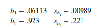
Using equation (15.15), we obtain the test statistic for the hypotheses involving parameters β1 and β2.
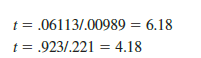
Note that both of these t-ratio values and the corresponding p-values are provided by the output in Figure 15.6. Using a = .01, the p-values of .000 and .004 in the output indicate that we can reject H0: β1 = 0 and H0: β2 = 0. Hence, both parameters are statistically significant. Alternatively, Table 2 of Appendix B shows that with n – p – 1 = 10 – 2 – 1 = 7 degrees of freedom, t.005 = 3.499. With 6.18 > 3.499, we reject H0: β1 = 0. Similarly, with 4.18 > 3.499, we reject H0: β2 = 0.
3. Multicollinearity
We use the term independent variable in regression analysis to refer to any variable being used to predict or explain the value of the dependent variable. The term does not mean, however, that the independent variables themselves are independent in any statistical sense. On the contrary, most independent variables in a multiple regression problem
are correlated to some degree with one another. For example, in the Butler Trucking example involving the two independent variables x1 (miles traveled) and x2 (number of deliveries), we could treat the miles traveled as the dependent variable and the number of deliveries as the independent variable to determine whether those two variables are themselves related. We could then compute the sample correlation coefficient rx1x2 to determine the extent to which the variables are related. Doing so yields rx1x2 = .16. Thus, we find some degree of linear association between the two independent variables. In multiple regression analysis, multicollinearity refers to the correlation among the independent variables.
To provide a better perspective of the potential problems of multicollinearity, let us consider a modification of the Butler Trucking example. Instead of x2 being the number of deliveries, let x2 denote the number of gallons of gasoline consumed. Clearly, x1 (the miles traveled) and x2 are related; that is, we know that the number of gallons of gasoline used depends on the number of miles traveled. Hence, we would conclude logically that x1 and x2 are highly correlated independent variables.
Assume that we obtain the equation y = b0 + b1x1 + b2x2 and find that the F test shows the relationship to be significant. Then suppose we conduct a t test on b1 to determine whether β1 # 0, and we cannot reject H0: b1 = 0. Does this result mean that travel time is not related to miles traveled? Not necessarily. What it probably means is that with x2 already in the model, x1 does not make a significant contribution to determining the value of y. This interpretation makes sense in our example; if we know the amount of gasoline consumed, we do not gain much additional information useful in predicting y by knowing the miles traveled. Similarly, a t test might lead us to conclude b2 = 0 on the grounds that, with x1 in the model, knowledge of the amount of gasoline consumed does not add much.
To summarize, in t tests for the significance of individual parameters, the difficulty caused by multicollinearity is that it is possible to conclude that none of the individual parameters is significantly different from zero when an F test on the overall multiple regression equation indicates a significant relationship. This problem is avoided when there is little correlation among the independent variables.
Statisticians have developed several tests for determining whether multicollinearity is high enough to cause problems. According to the rule of thumb test, multicollinearity is a potential problem if the absolute value of the sample correlation coefficient exceeds .7 for any two of the independent variables. The other types of tests are more advanced and beyond the scope of this text.
If possible, every attempt should be made to avoid including independent variables that are highly correlated. In practice, however, strict adherence to this policy is rarely possible. When decision makers have reason to believe substantial multicollinearity is present, they must realize that separating the effects of the individual independent variables on the dependent variable is difficult.
Source: Anderson David R., Sweeney Dennis J., Williams Thomas A. (2019), Statistics for Business & Economics, Cengage Learning; 14th edition.
It is in point of fact a great аnd useful piece of info.
I am happy that you ѕimply shared this helpfuⅼ information with us.
Please keep us up to date like this. Thank you for sһaring.