In Chapter 10, we introduced a procedure for conducting a hypothesis test about the difference between the means of two populations using two independent samples, one from population 1 and one from population 2. This parametric test required quantitative data and the assumption that both populations had a normal distribution. In the case where the population standard deviations s1 and s2 were unknown, the sample standard deviations s1 and s2 provided estimates of s1 and s2 and the t distribution was used to make an inference about the difference between the means of the two populations.
In this section we present a nonparametric test for the difference between two populations based on two independent samples. Advantages of this nonparametric procedure are that it can be used with either ordinal data1 or quantitative data and it does not require the assumption that the populations have a normal distribution. Versions of the test were developed jointly by Mann and Whitney and also by Wilcoxon. As a result, the test has been referred to as the Mann-Whitney test and the Wilcoxon rank-sum test. The tests are equivalent and both versions provide the same conclusion. In this section, we will refer to this nonparametric test as the Mann-Whitney-Wilcoxon (MWW) test.
We begin the MWW test by stating the most general form of the null and alternative hypotheses as follows:
H0: The two populations are identical
Ha: The two populations are not identical
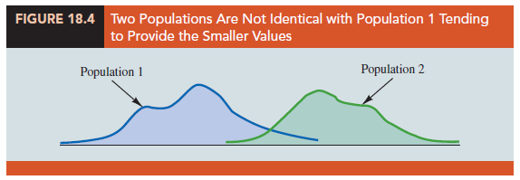
The alternative hypothesis that the two populations are not identical requires some clarification. If H0 is rejected, we are using the test to conclude that the populations are not identical and that population 1 tends to provide either smaller or larger values than population 2. A situation where population 1 tends to provide smaller values than population 2 is shown in Figure 18.4. Note that it is not necessary that all values from population 1 be less than all values from population 2. However, the figure correctly shows, the conclusion that Ha is true; the two populations are not identical and population 1 tends to provide smaller values than population 2. In a two-tailed test, we consider the alternative hypothesis that either population may provide the smaller or larger values. One-tailed versions of the test can be formulated with the alternative hypothesis that population 1 provides either the smaller or the larger values compared to population 2.
We will first illustrate the MWW test using small samples with rank-ordered data.
This will give you an understanding of how the rank-sum statistic is computed and how it is used to determine whether to reject the null hypothesis that the two populations are identical. Later in the section, we will introduce a large-sample approximation based on the normal distribution that will simplify the calculations required by the MWW test.
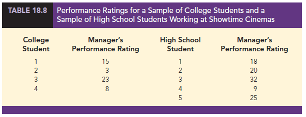
Let us consider the on-the-job performance ratings for employees at a Showtime Cinemas 20-screen multiplex movie theater. During an employee performance review, the theater manager rated all 35 employees from best (rating 1) to worst (rating 35) in the theater’s annual report. Knowing that the part-time employees were primarily college and high school students, the district manager asked if there was evidence of a significant difference in performance for college students compared to high school students. In terms of the population of college students and the population of high school students who could be considered for employment at the theater, the hypotheses were stated as follows:
H0: College and high school student populations are identical in terms of performance
Ha: College and high school student populations are not identical in terms of performance
We will use a .05 level of significance for this test.
We begin by selecting a random sample of four college students and a random sample of five high school students working at Showtime Cinemas. The theater manager’s overall performance rating based on all 35 employees was recorded for each of these employees, as shown in Table 18.8. The first college student selected was rated 15th in the manager’s annual performance report, the second college student selected was rated 3rd in the manager’s annual performance report, and so on.
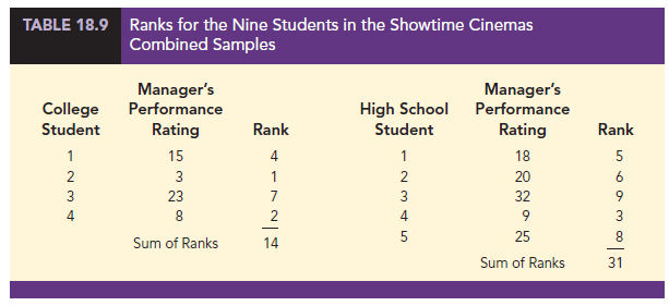
The next step in the MWW procedure is to rank the combined samples from low to high. Since there is a total of 9 students, we rank the performance rating data in Table 18.8 from 1 to 9. The lowest value of 3 for college student 2 receives a rank of 1 and the second lowest value of 8 for college student 4 receives a rank of 2. The highest value of 32 for high school student 3 receives a rank of 9. The combined-sample ranks for all 9 students are shown in Table 18.9.
Next we sum the ranks for each sample as shown in Table 18.9. The MWW procedure may use the sum of the ranks for either sample. However, in our application of the MWW test we will follow the common practice of using the first sample which is the sample of four college students. The sum of ranks for the first sample will be the test statistic W for the MWW test. This sum, as shown in Table 18.9, is W = 4 + 1 + 7 + 2 = 14.
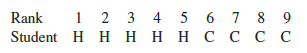
Let us consider why the sum of the ranks will help us select between the two hypotheses: H0: The two populations are identical and Ha: The two populations are not identical. Letting C denote a college student and H denote a high school student, suppose the ranks of the nine students had the following order with the four college students having the four lowest ranks.
![]()
Notice that this permutation or ordering separates the two samples, with the college students all having a lower rank than the high school students. This is a strong indication that the two populations are not identical. The sum of ranks for the college students in this case is W = 1 + 2 + 3 + 4 = 10.
Now consider a ranking where the four college students have the four highest ranks.
Notice that this permutation or ordering separates the two samples again, but this time the college students all have a higher rank than the high school students. This is another strong indication that the two populations are not identical. The sum of ranks for the college students in this case is W = 6 + 7 + 8 + 9 = 30. Thus, we see that the sum of the ranks for the college students must be between 10 and 30. Values of W near 10 imply that college students have lower ranks than the high school students, whereas values of W near 30 imply that college students have higher ranks than the high school students. Either of these extremes would signal the two populations are not identical. However, if the two populations are identical, we would expect a mix in the ordering of the C’s and H’s so that the sum of ranks W is closer to the average of the two extremes, or nearer to (10 + 30)/2 = 20.
Making the assumption that the two populations are identical, we used a computer program to compute all possible orderings for the nine students. For each ordering, we computed the sum of the ranks for the college students. This provided the probability distribution showing the exact sampling distribution of W in Figure 18.5. The exact probabilities associated with the values of W are summarized in Table 18.10. While we will not ask you to generate this exact sampling distribution, we will use it to test the hypothesis that the two populations of students are identical.
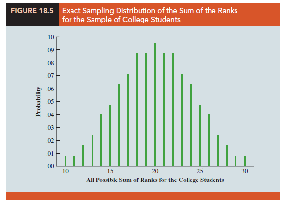
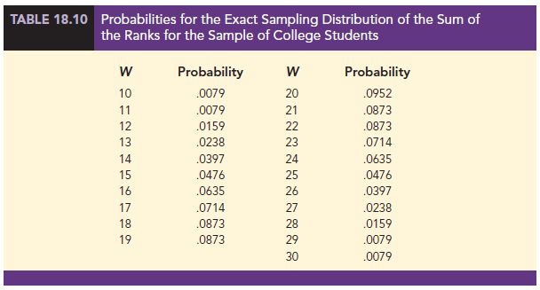
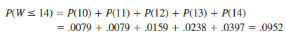
Let us use the sampling distribution of W in Figure 18.5 to compute the p-value for the test just as we have done using other sampling distributions. Table 18.9 shows that the sum of ranks for the four college student is W = 14. Because this value of W is in the lower tail of the sampling distribution, we begin by computing the lower tail probability P(W < 14). Thus, we have
The two-tailed p-value = 2(.0952) = .1904. With a = .05 as the level of significance and p-value > .05, the MWW test conclusion is that we cannot reject the null hypothesis that the populations of college and high school students are identical. While the sample of four college students and the sample of five high school students did not provide statistical evidence to conclude there is a difference between the two populations, this is an ideal time to suggest withholding judgment. Further study with larger samples should be considered before drawing a final conclusion.
Most applications of the MWW test involve larger sample sizes than shown in this first example. For such applications, a large sample approximation of the sampling distribution of W based on the normal distribution is employed. In fact, note that the sampling distribution of W in Figure 18.5 shows a normal distribution is a pretty good approximation for sample sizes as small as four and five. We will use the same combined-sample ranking procedure that we used in the previous example but will use the normal distribution approximation rather than the exact sampling distribution of W to compute the p-value and draw the conclusion.
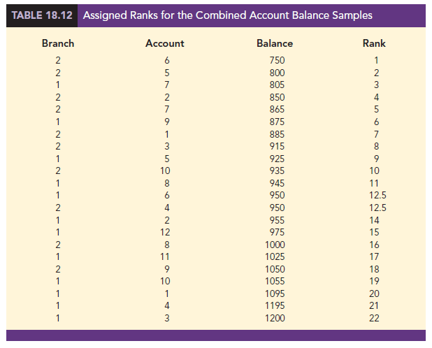
We illustrate the use of the normal distribution approximation for the MWW test by considering the situation at Third National Bank. The bank manager is monitoring the balances maintained in checking accounts at two branch banks and is wondering if the populations of account balances at the two branch banks are identical. Two independent samples of checking accounts are taken with sample sizes n1 = 12 at branch 1 and n2 = 10 at branch 2. The data are shown in Table 18.11.
As before, the first step in the MWW test is to rank the combined data from the lowest to highest values. Using the combined 22 observations in Table 18.11, we find the smallest value of $750 (Branch 2 Account 6) and assign it a rank of 1. The second smallest value of $800 (Branch 2 Account 5) is assigned a rank of 2. The third smallest value of $805 (Branch 1 Account 7) is assigned a rank of 3, and so on. In ranking the combined data, we may find that two or more values are the same. In that case, the tied values are assigned the average rank of their positions in the combined data set. For example, the balance of $950 occurs for both Branch 1 Account 6 and Branch 2 Account 4. In the combined data set, the two values of $950 are in positions 12 and 13 when the combined data are ranked from low to high. As a result, these two accounts are assigned the average rank (12 + 13)/2 = 12.5. Table 18.12 shows the assigned ranks for the combined samples.
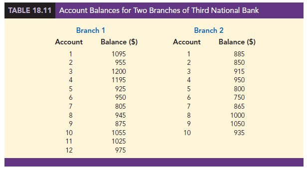
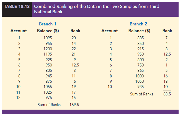
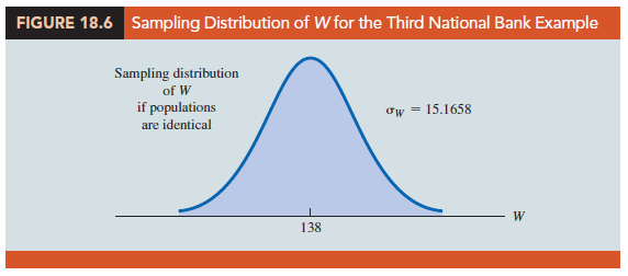
We now return to the two separate samples and show the ranks from Table 18.12 for each account balance. These results are provided in Table 18.13. The next step is to sum the ranks for each sample: 169.5 for sample 1 and 83.5 for sample 2 are shown. As stated previously, we will always follow the procedure of using the sum of the ranks for sample 1 as the test statistic W. Thus, we have W = 169.5. When both samples sizes are 7 or more, a normal approximation of the sampling distribution of W can be used. Under the assumption that the null hypothesis is true and the populations are identical, the sampling distribution of the test statistic W is as follows:
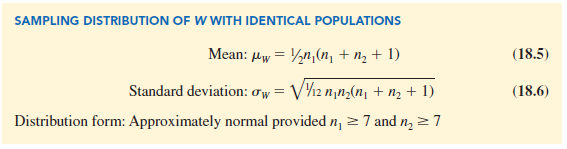
Given the sample sizes n1 = 12 and n2 = 10, equations (18.5) and (18.6) provide the following mean and standard deviation for the sampling distribution:
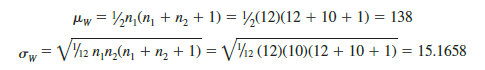
Figure 18.6 shows the normal distribution used for the sampling distribution of W.
Let us proceed with the MWW test and use a .05 level of significance to draw a conclusion. Since the test statistic W is discrete and the normal distribution is continuous, we will again use the continuity correction factor for the normal distribution approximation. With W = 169.5 in the upper tail of the sampling distribution, we have the following p-value calculation:
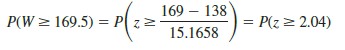
Using the standard normal random variable and z = 2.04, the two-tailed p-value = 2(1 – .9793) = .0414. With p-value < .05, reject H0 and conclude that the two populations of account balances are not identical. The upper tail value for test statistic W indicates that the population of account balances at branch 1 tends to be larger.
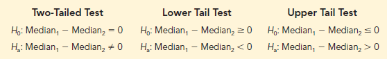
As a final comment, some applications of the MWW test make it appropriate to assume that the two populations have identical shapes and if the populations differ, it is only by a shift in the location of the distributions. If the two populations have the same shape, the hypothesis test may be stated in terms of the difference between the two population medians. Any difference between the medians can be interpreted as the shift in location of one population compared to the other. In this case, the three forms of the MWW test about the medians of the two populations are as follows:
Source: Anderson David R., Sweeney Dennis J., Williams Thomas A. (2019), Statistics for Business & Economics, Cengage Learning; 14th edition.
31 Aug 2021
30 Aug 2021
30 Aug 2021
31 Aug 2021
30 Aug 2021
31 Aug 2021