Factor Variables and Analysis of Covariance (ANCOVA) by using Stata

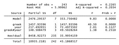
anova and many other Stata estimation commands allow independent variables specified in factor variable notation. The prefix i. written before the name of an independent variable tells Stata to include indicator (binary) variables for levels of a categorical variable, as if each category comprised its own dichotomous predictor. Categorical variables marked by the i. prefix must have non-negative integer values, from 0 to 32,740. anova by default views all independent variables as categorical, so typing

. anova drink greek year greek#year

invokes the same model as typing

. anova drink i.greek i.year i.greek#i.year

As often the case with ANOVA, we could get a more direct view of the underlying model by re-expressing the analysis as regression. Stata does this easily: simply type regress with no arguments immediately after anova.

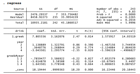
Note that sums of squares, F test, R² and other details are identical for these equivalent anova and regress analyses. The regress table gives more detail, however. We see that each value of year is treated as its own predictor. First-year college students form the omitted category in this table, so the coefficients on years 2, 3 and 4 express contrasts with these first-year students. Second-year non-Greek students drink somewhat more (+1.14), whereas fourth-year non-Greek students drink considerably less (-3.04) compared with first-year students. These year coefficients correspond to coefficients on dummy variables coded 1 for that particular year and 1 for any other. The greek coefficient corresponds to the coefficient on a dummy variable coded 1 for Greek and 0 for non-Greek students.

Analysis of covariance (ANCOVA) extends A-way ANOVA to encompass a mix of categorical and continuous x variables. The c. prefix identifies an independent variable as continuous, in which case its values are treated as measurements rather than separate, unordered categories. We might have treated year as continuous: . anova drink i.greek c.year i.greek#c.year

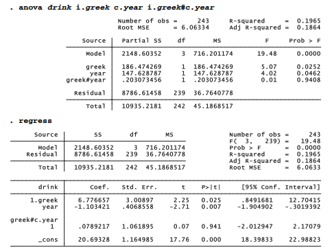
This version with year as continuous variable (c.year) instead of a categoricatl variable (i.year) results in a simpler model with more degrees of freedom, but the adjusted R² shows the continuous version does not fit as well (.1864 versus .2034 ). The categorical version found that drinking is higher (+1.14) in year 2 compared with year 1, slightly higher (+.36) in year 3 compared with year 1, but much lower (-3.04) in year 4 compared with year 1. The continuous version just smoothed the up-and-down details into an average decrease of -1.10 per year.

Treating year as a continuous or categorical variable can be the analyst’s call, based on substantive or statistical reasoning. Other variables such as student grade point average (gpa) are unambiguously continuous, however. When we include gpa among the independent variables, we find that it, too, is related to drinking behavior. This model omits the interaction effects, which have not proven to be significant. Because categorical variables are the default for anova, the i. prefixes can be omitted with greek and gender.

From this analysis we know that a significant relationship exists between drink and gpa when we control for greek and gender. Beyond their F tests for statistical significance, however, ANOVA or ANCOVA tables do not provide much descriptive information about how variables are related. Regression does a better job at this.

Source: Hamilton Lawrence C. (2012), Statistics with STATA: Version 12, Cengage Learning; 8th edition.