Bar Charts for Multiple Comparisons by using Stata

The catplot bar charts in Figure 4.3 depict a relationship between two categorical variables, each with four categories. If we have more than two variables, or more than a few categories, however, the catplot approach becomes cluttered. A cleaner alternative for making multiple comparisons of categorical variables employs Stata’s horizontal bar chart command hbar.

Figure 3.13 in the previous chapter tracked changes in the late-summer area of Arctic sea ice, over the years 1979-2011. The dramatic decline has attracted much scientific attention, and been widely noted in popular news media as well. Our Granite State Poll included a carefully worded question (warmice) testing whether people know about this. As with warmop, the order of response choices was rotated to avoid bias. A large majority (71%) know that ice area declined.

Which of the following three statements do you think is more accurate?

Over the past few years, the ice on the Arctic Ocean in late summer …

Covers less area than it did 30 years ago.

Declined but then recovered to about the same area it had 30 years ago.

Covers more area than it did 30 years ago.

. svy: tab warmice, percent ci

The warmice question allows four response choices, including “don’t know” or no answer. For some purposes, however, it proves useful to create a new dichotomous variable that just indicates whether they answered this question correctly. Variable warmiceQ equals 1 for respondents who said that ice area declined, and 0 for everyone else. About 71% answered correctly that late-summer sea ice covers less area than it did 30 years ago.

The mean of a {0,1} variable like warmiceQ simply equals the proportion of 1’s. Such {0,1} dummy variables have many uses in statistical modeling. For graphical purposes we might temporarily re-scale warmiceQ to have values of 0 or 100 instead. The mean of a {0,100} variable equals the percentage of 100s, or the percentage of correct answers on Arctic ice in this example. By applying graph hbar to a {0,100} dichotomy, we can visually compare many different percentages. The bar chart in Figure 4.4 gives the weighted percent of correct answers among college graduates and others (variable college).

Note that in Stata’s horizontal bar charts (graph hbar; also in graph hbox and some other turned-sideways graphics) the horizontal axis is called the y axis, contrary to usual convention. Thus ytitle(“Weighted percent”) specifies a title that goes along the bottom. Stata does not recognize an x axis in these charts, although l1title( ) could specify a title that would go along the left-hand side.

Figure 4.4 compared only two numbers, 76% among college graduates and 64% among others. No one needs to draw a graph to make such a simple comparison. This bar-chart approach readily extends to more complicated comparisons, however. Previous surveys have found pervasive partisan divisions across many questions involving climate change. Might those exist even for this factual question about Arctic sea ice? A three-variable bar chart in Figure 4.5 gives the percent of correct answers broken down by college education and respondent’s political identification (variable party).

. graph hbar (mean) warmiceQ100 [aw = censuswt],

over(college) over(party)

blabel(bar, format(%3.0f)) ytitle(“Weighted percent”)

title(“Arctic ice declined, by college and political party”

, size(medium))

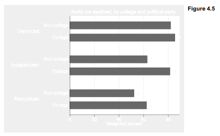
Within each party group we see a college-education effect, and within each level of education we see a partisan difference as well.

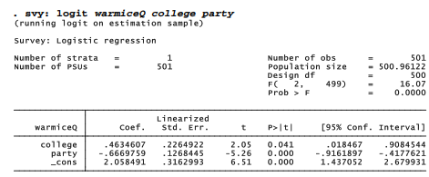
Figure 4.5 cannot tell us whether the differences are statistically significant. Answering that question requires statistical modeling tools introduced in Chapter 9. As a preview, however, the following weighted logit regression model confirms that both college and party have statistically significant effects, positive in the case of college (0 = non-college, 1 = college grad) and negative in the case of party (1 = Democrat, 2 = Independent, 3 = Republican). Party is a stronger predictor than college.

Chapter 9 will return to this example, applying a statistical method (multinomial logit) that can model the predictors of each separate answer to the ice-area question.

Source: Hamilton Lawrence C. (2012), Statistics with STATA: Version 12, Cengage Learning; 8th edition.