Simple Regression by using Stata

File Nations2.dta contains U.N. human-development indicators for 194 countries: . use C:\data\Nations2.dta, clear

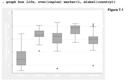
Life expectancies (life) exhibit much place-to-place variation. For example, Figure 7.1 shows that they tend to be lower in Africa than elsewhere.

To what extent can variations in life expectancy be explained by average education, per capita wealth and other development indicators? We might begin to study education effects by conducting a simple regression of life expectancy on mean years of schooling. Basic syntax for Stata’s regression command is regressy x, where y is the predicted or dependent variable, and x the predictor or independent variable.

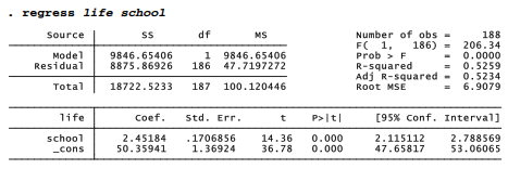
As might be expected, life expectancies tend to be higher in countries with higher levels of schooling. A causal interpretation is premature at this point, but the regression table conveys information about the linear statistical relationship between life and school. At upper right it gives an overall F test, based on the sums of squares at the upper left. This F test evaluates the null hypothesis that coefficients on all x variables in the model (here there is only one x variable, school) equal zero. The F statistic, 206.34 with 1 and 186 degrees of freedom, leads easily to rejection of this null hypothesis (p = .0000 to four decimal places, meaning p < .00005). Prob > F means “the probability of a greater F statistic” if we drew many random samples from a population in which the null hypothesis is true.

At upper right, we also see the coefficient of determination, R² = .5259. Schooling explains about 53% of the variance in life expectancies. Adjusted R², R²_a = .5234, takes into account the complexity of the model relative to the complexity of the data.

The lower half of the regression table gives the fitted model itself. We find coefficients (slope and y-intercept) in the first column. The coefficient on school is 2.45184, and the y-intercept (listed as the coefficient on _cons) is 50.35941. Thus our regression equation is approximately predicted life = 50.36 + 2.45school

For every additional year of mean schooling, predicted life expectancy rises 2.45 years. This equation predicts a life expectancy of 50.36 years for a country where the mean schooling is zero — although the lowest value in the data is 1.15 years of schooling (Mozambique).

The second column lists estimated standard errors of the coefficients. These are used to calculate t tests (columns 3-4) and confidence intervals (columns 5-6) for each regression coefficient. The t statistics (coefficients divided by their standard errors) test null hypotheses that the corresponding population coefficients equal zero. At the a = .05 or .001 significance levels, we could reject this null hypothesis regarding both the coefficient on school and the y-intercept; both probabilities show as “.000” (meaningp < .0005). Stata’s modeling procedures ordinarily show 95% confidence intervals, but we can request other levels by specifying the level( ) option. For example, to see 99% confidence intervals instead, type
. regress life school, level(99)

After fitting a regression model, we could re-display the results just by typing regress, without arguments. Typing regress, level(90) would repeat the results but show 90% confidence intervals this time. Because the Nations2.dta dataset used in these examples does not represent a random sample from some larger population of nations, hypothesis tests and confidence intervals lack their literal meanings.

Mean years of schooling among these nations range from 1.15 to 12.7. What mean life expectancies does our model predict for nations with, for example, 2 or 12 years of schooling? The margins command offers a quick way to view predicted means along with their confidence intervals, and z tests (which often are not interesting) for whether those means differ from zero. A “vertical squish” vsquish option reduces the number of blank lines between rows in the table.

At school = 2, predicted mean life expectancy equals 55.26 years, with a confidence interval from 53.19 to 57.34. At school = 12, predicted mean life expectancy is 79.78 years with an interval from 77.97 to 81.59. We could obtain predicted means of life expecting for school values at 1-year intervals from 2 through 12, and graph the results, by typing two commands:

. margins, at(school = (2(1)12)) vsquish

. marginsplot

In regression tables, the term _cons stands for the regression constant, usually set at one (so the coefficient on _cons equals the y intercept). Stata automatically includes a constant unless we tell it not to. A nocons option would cause Stata to suppress the constant, performing regression through the origin:

. regress y x, nocons

For some applications you might wish to specify your own constant. If the right-hand side variables include a user-supplied constant (named c, for example), employ the hascons option instead of nocons:

. regress y c x, hascons

Using nocons in this situation would result in a misleading F test and R². Consult the Base Reference Manual or help regress for more about hascons.

Regression with one predictor amounts to finding a straight line that best fits the scatter of data, with “best fit” defined by the ordinary least squares (OLS) criterion. An easy way to graph this line is to draw a scatterplot (twoway scatter) overlaid with the a linear fit (lfit) plot. The command below would draw a basic version (not shown),

Figure 7.2 displays a nicer version, suppressing the unneeded legend, and inserting the regression equation as text. The variable names life and school illustrate how to italicize text in Stata graphs.

Source: Hamilton Lawrence C. (2012), Statistics with STATA: Version 12, Cengage Learning; 8th edition.