Further rreg and qreg Applications by using Stata

The previous section showed basic applications of rreg and qreg. These commands also can be used in many other ways, from simple to complex. For example, to obtain a 90% confidence interval for the mean of a single variable such as Antarctic air temperature (tempS), we could type the usual confidence-interval command ci:

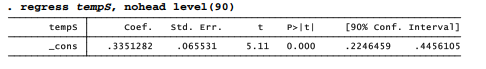
Alternatively, we could get exactly the same mean and interval through a regression with no x variables. The nohead option suppresses the top of a regression table, which is not needed here.

Similarly, we can obtain a robust mean with 90% confidence interval. nolog suppresses the robust iteration log here to save space.

qreg could be used in the same way to obtain approximate confidence intervals for one or more medians, with the caveat that a .5 quantile found by qreg might not exactly equal a sample median. In theory, .5 quantiles and medians are the same. In practice, quantiles are approximated from actual sample data values, whereas the median is calculated by averaging the two central values, if a subgroup contains an even number of observations. The sample median and .5 quantile approximations then can be different, but in a way that does not much affect model interpretation.

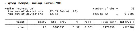
The robust mean is slightly lower than the ordinary mean (.319 versus .335), and the .5 quantile (.28) is lower than either — suggesting that a few warm years are pulling the mean up. In any of these commands, the level( ) option specifies the desired degree of confidence. If we omit this option, Stata automatically displays a 95% confidence interval.

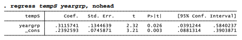
To compare two means, analysts typically employ a two-sample t test (ttest) or one-way analysis of variance (oneway or anova). As seen earlier, we can perform equivalent tests (yielding identical t and F statistics) by regressing the measurement variable on a dummy variable. The dummy variable yeargrp, coded 0 for years 1972-1999 and 1 for years 2000-2011, provides an illustration. Figure 8.8 graphs temperature anomalies for these two groups of years.

. graph box tempS, over(yeargrp)

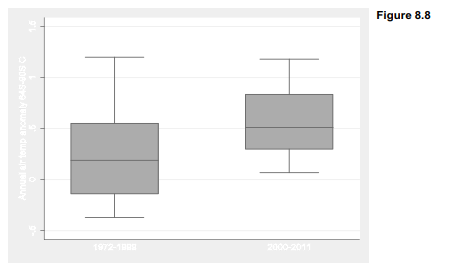
Regression analysis confirms the visual impression from Figure 8.8: later years are significantly (p = .026) warmer. The mean Antarctic temperature anomaly is .239 °C for 1992-1999, and .312 °C higher than that (.239 + .312 = .551 °C) for 2000-2011. It should be noted that even with half a degree of warming, Antarctica remains a very cold place. Temperatures that stay well below freezing year-round at the South Pole.

Is that conclusion robust? rreg finds that the robust means differ even more, by .329 °C. That difference too is significant (p = .023).

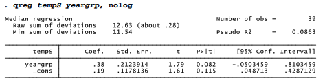
qreg finds that the .5 quantiles are even farther apart, .38 °C. This difference is not statistically significant, however (p = .082). The larger difference fails to reach statistical significance because the standard errors are much larger in the qreg analysis, resulting in a lower t statistic. A larger standard error reflects qreg’s relatively low efficiency.

.

With effect coding and suitable interaction terms, regress can duplicate ANOVA exactly. That is, regress followed by the appropriate test commands obtains exactly the same R² and F test results that would be obtained using anova. Predicted values from such regressions equal the group means. rreg can perform parallel analyses, testing for differences among robust means instead of ordinary means. Used in similar fashion, qreg opens the third possibility of testing for differences among medians. That allows us to fit models analogous to N-way ANOVA or ANCOVA, but involving .5 quantiles or approximate medians instead of the usual means.

Regardless of error distribution shape, OLS remains an unbiased estimator. Over the long run, its estimates should center on the true parameter values. The same is not true for most robust estimators. Unless errors are symmetrical, the median line fit by qreg, or the biweight line fit by rreg, does not theoretically coincide with the expected-y line estimated by regress. So long as the errors’ skew reflects only a small fraction of their distribution, rreg might exhibit little bias. But when the entire distribution is skewed, rreg will downweight mostly one side, resulting in noticeably biased y-intercept estimates. rreg slope estimates, however, remain unbiased despite skewed error distributions. Thus there is a tradeoff using rreg or similar estimators with skewed errors: we risk getting biased estimates of the y-intercept, but can still expect unbiased and relatively precise estimates of other regression coefficients. In many applications, such coefficients are substantively more interesting than the y-intercept, making the tradeoff worthwhile. Moreover, the robust t and F tests, unlike those of OLS, do not assume normal errors.

Source: Hamilton Lawrence C. (2012), Statistics with STATA: Version 12, Cengage Learning; 8th edition.