Robust Regression by using Stata

Stata’s basic regress and anova commands perform ordinary least squares (OLS) regression. The popularity of OLS derives in part from its theoretical advantages given ideal data. If errors are normally, independently and identically distributed (normal i.i.d.), then OLS is more efficient than any other unbiased estimator. The flip side of this statement often gets overlooked: if errors are not normal, or not i.i.d., then other unbiased estimators might outperform OLS. In fact, the efficiency of OLS degrades quickly in the face of heavy-tailed (outlier-prone) error distributions. Yet such distributions are common in many fields.

OLS tends to track outliers, fitting them at the expense of the rest of the sample. Over the long run, this leads to greater sample-to-sample variation or inefficiency when samples often contain outliers. Robust regression aims to achieve almost the efficiency of OLS with ideal data and substantially better-than-OLS efficiency in less ideal situations such as nonnormal errors. Robust regression encompasses a variety of different techniques, each with advantages and drawbacks for dealing with problematic data. This section introduces two varieties of robust regression, rreg and qreg, and briefly compares them with OLS (regress).

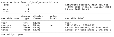
In Chapter 7 we noted a clear downward trend, steeper than linear, in the minimum area of Arctic sea ice over the years 1979-2011. What about Antarctic sea ice? Its geography and seasonal patterns are quite different. The central Arctic is an ocean surrounded by land, which even after the recent declines retained more than 3 million km² of area, or 4 million km² of extent (the area with at least 15% ice) at its summer minimum. The Antarctic, on the other hand, is land surrounded by ocean. Whereas Arctic sea ice extends to the North Pole, Antarctic sea ice exists at comparatively lower latitudes far from the South Pole. Most of the Antarctic sea ice melts every summer. At the annual minimum in February, Antarctic sea ice area falls to about 2 million km², and extent to less than 3 million km². Dataset Antarctic2.dta contains mean February sea ice extent data (Milke and Heygster 2009), covering the years 1972-2011. The dataset also contains annual air temperature anomalies for the Antarctic region, from 64 to 90 degrees south latitude, estimated by NASA.

Is minimum Antarctic sea ice extent trending up or down? OLS regression finds a weak and statistically nonsignificant downward trend (p = .125).

The Arctic decline was obvious in graphs (see Figures 7.9 or 7.12). A graph of the Antarctic decline in Figure 8.4 reveals no obvious trend. We do see potential statistical problems,
however. High extents values in 1972 and 1977, a period when satellite observations were less detailed, might be influencing the regression line and causing its weak negative slope.

Robust regression resists the pull of outliers, making it well suited for a quick check on whether outliers unduly affect our OLS results. The command rreg performs robust regression. Applied to Antarctic sea ice, rreg finds a decline that is slightly less steep, and also not significant.

After rreg, the predict command works as usual to obtain predicted values. Graphing these predicted values (here named exthatl), Figure 8.5 visually compares robust and OLS lines.

rreg works by iteratively reweighted least squares (IRLS). The first rreg iteration begins with OLS. Any observations so influential as to have Cook’s D values greater than 1 are automatically set aside after this first step. Next, weights are calculated for each observation using a Huber function (which downweights observations that have larger residuals) and weighted least squares is performed. After several WLS iterations, the weight function shifts to a Tukey biweight (as suggested by Li 1985), tuned for 95% Gaussian efficiency (see Hamilton 1992a for details). rreg estimates standard errors and tests hypotheses using a pseudovalues method (Street, Carroll and Ruppert 1988) that does not assume normality.

rreg and regress both belong to the family of M-estimators (for maximum-likelihood). An alternative order-statistic strategy called L-estimation fits quantiles of y, rather than its expectation or mean. For example, we could model how the median (.5 quantile) ofy changes with x. qreg (an L1 -type estimator) accomplishes such quantile regression. Like rreg, qreg has good resistance to outliers. However, qreg tends to be less efficient, or have higher standard errors, compared to rreg with most data. That is the case here: qreg finds an even shallower slope, but with greater standard errors. Figure 8.6 graphically compares all three linear models.

qreg performs median regression by default, but has more general capabilities. It can fit linear models for any quantile of y, not just the median (.5 quantile). For example, the following command finds that the third quartile (.75 quantile) of extents declines somewhat more steeply than the median does over time. The slope for .75 quantile is -.0149, meaning a decline of 14,900 km² per year, compared with just 5,600 km² per year for the .5 quantile or median. Neither trend is statistically significant, however.

Assuming constant error variance, the slopes of the .25 and .75 quantile lines should be roughly the same. qreg thus could perform a check for heteroskedasticity or subtle kinds of nonlinearity.

Like regress, both rreg and qreg can work with transformed variables (such as logarithms or squared terms) and with any number of predictors including dummy variables or interactions. Efficiency and ease of use make rreg particularly valuable as a quick, general check on whether regress results might be affected by outliers or non-normal error distributions. If rreg and regress, applied to the same model, obtain roughly similar results, then we can state our conclusions with more confidence. Conversely, if rreg and regress disagree, that presents a yellow flag warning us that our conclusions are unstable. Further investigation is needed to learn why they differ, and figure out what to do about the statistical problem this reveals.

The differences between regress, rreg and qreg results are not large in our Antarctic sea ice example. All three methods agree that there is a weak, statistically nonsignificant downward trend. regress gives a slightly steeper slope for this trend because it is more influenced by the high early years. The rreg or qreg models might be preferred for this reason, but we could also step back and ask whether a linear model is reasonable in the first place. Lowess regression, which does not assume any particular functional form, provides a good tool for exploring questions of this type. Applied to Arctic sea ice (not shown), lowess finds a curve very similar to the quadratic model in the last chapter’s Figure 7.12. Applied to Antarctic sea ice in Figure 8.7 below, however, lowess finds nothing resembling a linear or quadratic model. Instead, it suggests a qualitative description of initial decline, subsequent rebound, and perhaps a downturn in the last years. Only the initial decline appears large, and our interpretation there is complicated by limitations of the satellite record. Perhaps a longer-term pattern will become evident in years ahead, but one is not yet clear from these data.

Source: Hamilton Lawrence C. (2012), Statistics with STATA: Version 12, Cengage Learning; 8th edition.