How Do I Test a System?

Testing a hypothetical system is absolutely necessary, and the testing process can be tedious because so many ideas of how to trade turn out to be unsuccessful. This is the most difficult aspect of designing a system, and unfortunately, because it is so time-consuming and discouraging, many analysts take short-cuts, such as not performing out-of-sample tests, and end up with a system that eventually blows up on them. The process begins with being sure the data being used in the testing is clean and the same as the data that will be used later when the system goes live. The next is to establish the rules for the model being chosen as the basis for the system and optimize the variables chosen. These rules include entry and exit signals at first and will have other filters added later depending on the results of the first series of tests. If a walk-forward program is not available, a large portion of the data, called out-of-sample data, must be kept aside to use later when testing the system for robustness. Once a viable system has been adequately optimized, the resulting parameters are then tested against the out-of-sample data to see if the system works with unknown data and was not the result of curve-fitting or data mining. This is the disheartening part of system design because invariably the out-of-sample test will fail, and the development must return to the beginning. It is at this point that most amateurs give up.

1. Clean Data

Not surprisingly, for an accurate evaluation of any system, the data must be impeccable. Without the correct data, the system tests are useless. Data should always be the same as what will be used when the system is running in real time. Not only the data but also the data vendor should be the same source as what will be used in practice. Different vendors receive different data feeds. This is especially a problem in short-term systems, where the sequence of trades is important for execution and for pattern analysis.

The amount of data required depends on the period of the system. A general rule of thumb is that the data must be sufficient to provide at least 30 to 50 trades (entry and exit) and cover periods where the market traveled up, down, and sideways. This will ensure that the test has enough history behind it and enough exposure to different market circumstances.

The real-time trader has enough difficulty with “dirty” data on a live feed, and this becomes just as crucial when testing back data. Cleanliness of data is a necessary requirement. Any anomalies or mispriced quotes will have an effect on the system test and will skew the results in an unrealistic manner. Cleaning of data is not an easy task and often must be relegated to the professional data providers.

2. Special Data Problems for Futures Systems

Although stock data has a few historical adjustments such as dividend payments, splits, offerings, and so on, the futures market has another more serious problem: which contract to test. Most futures contracts have a limited life span that is short enough not to be useful in testing most systems. The difficulty comes from the difference in price between the price at expiration and the price of the nearest contract on that date into which the position would be rolled. Those prices are rarely the same and are difficult to splice into something realistic that can be used for longer-term price analysis. To test a daily system, for example, two years or more of daily data is required at the very least, but no contract exists that runs back for two years. Of course, testing can be done on nearest contract series, but it is limited to the contract length. This is satisfactory if the system trades minute by minute but not for daily signals in a longer-term system.

To rectify this problem, two principal methods of splicing contract prices of different expirations together in a continuous stream have been used. These methods are known as perpetual contracts and continuous contracts. Neither is perfect, but these methods are the ones most commonly used in longer-term price studies.

Perpetual contracts, also called constant forward contracts, are interpolations of the prices of the nearest two contracts. Each is weighted based on the proximity to expiration of the nearest contract to the forward date—say, a constant 90 days. As an example, assume that today is early December, only a few days from expiration of the December contract of a commodity future and a little over three months from the expiration of the March contract, the next nearest. The 90-day perpetual would be calculated by proportioning each contract’s current price by the distance each is in time from the date 90 days from now. This weighting in early December favors the March contract price, and each day as we approach the December expiration, the December contract receives less weight until expiration when the perpetual is just the March contract price. The following day, however, the March contract price begins to lose weighting as the June contract price begins to increase its weighting. This process gives a smooth but somewhat unrealistic contract price; it eliminates the problem of huge price gaps at rollover points, but you cannot literally trade a constant forward series. As Schwager points out, “the price pattern of a constant-forward series can easily deviate substantially from the pattern exhibited by the actual traded contracts—a highly undesirable feature” (1996, p. 664).

The continuous, or spread-adjusted, contract is more realistic, but it suffers from the fact that at no time is the price of the continuous contract identical to the actual price because it has been adjusted at each expiration or each rollover date. The continuous contract begins at some time in the past with prices of a nearby contract. A rollover date is determined based on the trader’s usual rollover date—say, ten days before expiration. Finally, a cumulative adjustment factor is determined. As time goes on and different contracts roll over to the next contract, this spread between contracts is accumulated and the continuous contract price adjusted accordingly. With this method, the continuous prices are exactly what would have been the cost to the trader had the system signals been followed when they occurred. There is no distortion of prices. Price trends and formations occur just as they would have at the time. The only difference is that the actual prices are not those in the continuous contract. Percentage changes, for example, are not accurate. Nevertheless, the method demonstrates exactly what would have happened to a system during the period of the continuous contract, which is precisely what the systems designer wants to know.

As Schwager points out, “a linked futures price series can only accurately reflect either price levels, as does the nearest futures, or price moves as does continuous futures, but not both…” (1996, p. 669). Students interested in trading futures can refer to the book Schwager on Futures: Technical Analysis, to learn more about these techniques.

3. Testing Methods and Tools

Fortunately, the wheel need not be reinvented when it comes to testing software. Many trading software products include a testing section. Some are reliable; however, some are not. Before purchasing any such software, you should understand the testing methods and resulting reports of the software. Almost all such programs leave out crucial analysis data and may often define terms and formulas differently from others. For example, the term drawdown has different meanings, depending on intraday data, closing data, trade close data, and so forth. You must understand the meaning of all terms in any software program to correctly interpret tests performed by it. With this in mind, the systems analyst must establish exactly what information is desired, what evaluation criteria would be useful, and how the results should be presented.

4. Test Parameter Ranges

The initial test of a system is run to see if the system has any value and, if so, where the problem areas might lie. When the testing program is run, the parameters selected initially should be tested to see if they fall in a range or are independent spikes that might or might not occur in the future. A parameter range, called the parameter set, which gives roughly the same results, bolsters confidence in the appropriateness of the parameter value. If, when the parameter value is changed slightly, the performance results deteriorate rapidly, the parameter will not likely work in the future. It is just an aberration. When the results remain the same or similar, the parameter set is said to be stable—obviously a desirable characteristic.

Box 22.1 Designing a System: “HAL” (Name of the Computer in 2001: A Space Odyssey)

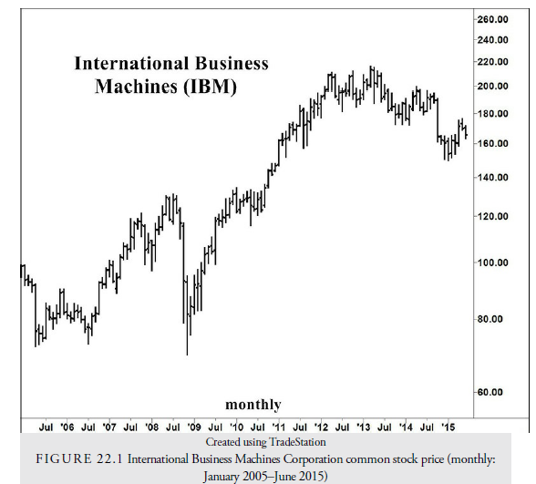
Let us look at a simple case study of how to develop a trading system. Suppose we decide that we will trade International Business Machines (IBM), traditionally a less volatile blue chip.

We also decide that we will start with an oscillator called the Commodity Channel Index (CCI). The CCI is an oscillator similar to the Stochastic only it includes a volatility component and thus makes it a more realistic indicator of overbought or oversold. The signals will come from the CCI crossing levels determined by the optimization.

Looking at the monthly chart of IBM (see Figure 22.1) from 2005 through mid-2015, we see several periods of upward and downward trends and trading ranges. This is an ideal history to analyze and test because it includes the three possible trends in any market: up, down, and sideways. It also covers a period of more than nine years, roughly 2250 days, enough to give us plenty of signals.

Normally the CCI is contained with +300 and -300 but is not explicitly bounded. The only variables are the length of the moving averages used in its construction and the level of the two signal lines.

The account will assume a capitalization of $30,000, and commissions and slippage will be 10 cents per share for each entry and exit or 20 cents per share total. The entries will be limited to 100 shares per trade and only one 100-share position allowed. The reason for this model in our exercise is that we know it has worked well over the past two years, and we want to see if changing the parameters can improve its performance.

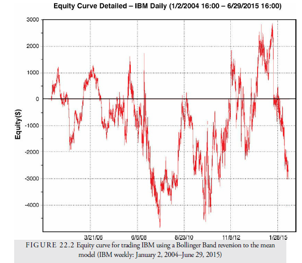
The equity curve for this system with the default length parameter of 14 and signal levels as + 100 and -100 is shown in Figure 22.2. An equity curve is a chart of the equity in the account (vertical axis) versus time measured either by trade number or by time (horizontal axis). In Figure 22.2, time is along the horizontal axis. Looking at the chart, we can see that the system had a mixed performance and could easily be discarded as just another oscillator. However, if we change the parameters through optimization and walk-forward testing, perhaps we can find a more reliable formula that worked in the past for the entire period and will have a good chance of working in the future.

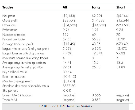
Let’s look at some of these statistics and learn what they tell us about the HAL system so far:

• Net profit is the difference between gross profit and gross loss. It is negative for this system as a whole but positive for long positions. This problem can be attacked in one of two ways: using different parameters for selling short or just using it for long signals. If we use long signals only, we already have a viable system that has worked in the past but not very well. We decide we will adjust both long and short signals with an optimization and walk-forward test.
• G ross profit and gross loss are the totals under each category for each trade. Gross profit is the total profit from profitable trades; gross loss is the total from all losing trades.
• The profit factor is the absolute value of the ratio of gross profit to gross loss. It shows the profitability of the system. In this case, for every dollar of loss, 0.94 dollars of profit are generated; in other words, it is a losing system. The long side only was favorable at 1.29. The better systems are above 2.00.
• Looking at the number of trades, this system generated 139 trades: 69 long trades and 70 short trades. This is a large enough number of trades for reliable statistics. Generally, at least 30–50 trades are required to test a system.
• Percent profitable is the percent of all trades that were profitable. In our example, 57.55% of the trades were profitable, yet the system lost money. This suggests that there is something wrong with the losing trades; although fewer in number, they are losing more than the winners.
• Average trade net profit is the average profit received per trade. This is negative and suggests that the system is vulnerable to transaction costs.
• The largest winner or loser versus gross profit or gross loss figure gives a hint as to whether the gain or loss was accounted for by only one trade. In this case, the largest winning trade accounted for 5.92% of the total gross profit. This is a reasonable size when considering that the total number of trades was greater than 139.
• The maximum consecutive losing trades is important because a long string of consecutive losses invariably causes a large drawdown and, thus, a high potential risk for the system. In this case, the number of successive losses is four trades in a row. It suggests that two whipsaws took place during the test period. Whipsaws can be controlled with stops.
• Considering the average weeks in winning and losing positions, there is not much question that the HAL has a problem with losing trades. There should be considerably less time in losing trades. The rule of thumb is that one-quarter of the time can be spent on losing trades versus winning trades, but with a long holding period, the system isn’t kicking the losers out soon enough.
• Buy-and-hold return (80.7%) is the return gained if the investor bought the IBM on the first day and held it for the entire time period through all its gyrations. This is the number to beat.
• Return on account (-40.41%) is the total return on the minimum account size as determined by the maximum drawdown. It should be compared to the buy-and-hold return to see if the system outperforms a do-nothing approach. In this case, the system failed to exceed the do-nothing approach. Of course, such comparisons are not as easy as they look because the concept of risk has not been introduced to either method. The buy- and-hold method has infinite risk because the drawdown can be 100%. The risk of the system has been limited to a much smaller percentage, but we are still observing losses.
• Average monthly return and standard deviation of the monthly return are used to determine the volatility of returns. The average monthly return for this system is – $31.63, but it is highly volatile with a standard deviation of $887.80. Ideally, a system should have a standard deviation less than five times the monthly return. In this case, it is 31.5 times, far above the limit, and likely due to the large number of losses.
• The Sharpe ratio is a common measure of the return versus risk of a portfolio or As we saw in Chapter 21, “Selection of Markets and Issues: Trading and Investing,” it is a ratio of return—in this case, adjusted for the risk-free return of T-bills, to the standard deviation of return, a proxy for risk. As we stated earlier, however, risk is not just volatility, but is also the risk of capital loss. The Sharpe ratio fails to account for drawdown and fails to account for skewed deviations of return. An investment that deviates more to the upside, for example, will not be fairly represented by the Sharpe ratio, which assumes a normal distribution. These problems are why system designers shy away from the Sharpe ratio and have designed other ratios of return to risk that are more realistic. In this system, the Sharpe ratio is close to zero, suggesting that the return does not exceed the risk-free return of T-bills.
• SystemMAR is the ratio of annual percentage net gain for the system to the maximum percentage drawdown (MDD). The maximum percentage drawdown is the maximum percent that the equity curve corrected from a peak. The ratio measures the greatest decline that occurred during the system run and thus the potential loss in the future for the system. A ratio of greater than 1.0 is preferred. Naturally, one wants a system that has no drawdown, but barring that, one wants a system that has profits considerably higher than any drawdown potential. A large drawdown lowers trust in the system and may cause a premature close of the system before it has a chance to perform. The HAL has a negative gain versus a maximum drawdown. The favored standard is anything above 1.00. The ratio is, thus, a gauge for comparing systems.

• TradeMAR is the ratio of the net annual gain percentage to the largest trade drawdown in a trade, sometimes called the Maximum Adverse Excursion. Where maximum system drawdown may include many trades, the individual trade risk is also needed to gauge the systems performance and isolate where losses are occurring.

HAL may have promise if we can fix the problem with lengthy losing trades and the short selling losses. The long only section is satisfactory and will improve with improvement in the losses, but the entire system is bogged down by poor performance in the short side. This is not surprising in a market that has a generally upward trend, but it still is disappointing. We look next at ways to improve this system with optimized parameters and changes in the model logic.

Source: Kirkpatrick II Charles D., Dahlquist Julie R. (2015), Technical Analysis: The Complete Resource for Financial Market Technicians, FT Press; 3rd edition.