Once you determine that the parameters in your system are valid, you may optimize the system. Optimizing is simply changing the parameters of a system to achieve the best results. The most important benefit of optimization is that the designer may find parameters that do not work under any circumstances. If parameters do not work with the past data, it is highly likely they will not work in the future. Thus, optimizing can eliminate useless rules and parameters.
Optimizing is also useful in determining whether certain types of stops are useful. Often the designer finds that there is a limit—for example, to a protective stop—beyond which the stop does not add to the system performance. Often, the distance of trailing stops is too close to the last price, causing premature exits. These determinations can be analyzed more closely with optimization.
Although it can be beneficial, optimization does come with major hazards. With modern computers and sophisticated software, we can take any series of prices and find the best parameters for any predefined system. The problem is that by doing such an optimization, we are just fitting the data to a curve of results and have no idea whether the parameters we have derived will perform in the future. Because the future is what we are attempting to control, most optimization is useless and even dangerous because it gives us a false sense of confidence.
The principal concern with optimization is the tendency to curve-fit. Curve-fitting occurs when the optimization program finds the absolute best set of parameters. What the program is really doing is fitting the parameters to the data that is being tested. Thus, it is forming a mathematical model of that data and fitting parameters to that particular time in history. The only way that the parameters will work in the future is if the future exactly duplicates the history that was optimized. Of course, we know this will never happen and, thus, the parameters determined by optimization likely will be useless in the future. Any system could be made to look profitable if optimized; this is a problem that buyers of systems must face when considering purchasing an existing system for investing or trading. The trick is to optimize over a certain period and then test the parameters derived through optimization on a period in which no optimization has been conducted. This is called out-of-sample (OOS) testing. Invariably we will find that the results in the optimization will overstate the results in the out-of-sample period and, thus, the optimized parameters should never be used to evaluate the system’s usefulness. Optimization should be kept simple. Fine-tuning the system just increases the level of false confidence that eventually will be dashed in real time when the system fails.
There is, thus, some controversy about the use of optimization in arriving at workable mechanical systems. The basic principles of realistic optimization are to keep it simple, test out-of-sample data against in-sample optimization results, preferably use baskets of securities, determine parameter sets instead of single parameters, understand that the best results are high profits with minimal risk, and avoid expecting to find the Holy Grail. Next, we discuss some optimization methods and some tests for statistical significance to perform after the most realistic parameter sets have been determined.
Before optimizing, the analyst must decide what the optimization is looking for in the data. Is it looking for net profit, maximum drawdown, Sharpe ratio, percentage of winning trades, or any other objective function? This objective function is an important aspect of the investigation for the best system. What is best? Many analysts use as their objective function a ratio of net profit to maximum drawdown, called the MAR ratio, to account not only for profits but also for risk of loss. Others use a regression line fit to the resulting profits. A tight fit suggests less volatility and thus less drawdown. A variation is called the perfect profit correlation. It assumes that the perfect system would buy every trough and sell every peak and thus generate a certain “perfect” profit. The tested system results are then compared to the perfect system to see how well it correlated.
1. Methods of Optimizing
As a general rule, an optimization should be done over a considerable period of price data and include those periods when the prices are in trends and in trading ranges. We do not know ahead of time whether the future will be similar, but we do know that there will be trends and trading ranges. Any system must be able to deal with both of these situations and have developed adjustable parameter sets or rules that will account for them. Parameters determined in this manner should be suitable for future conditions.
2. Whole Sample
One method of optimizing is to take the entire price sample and run an optimization of the parameters. This is usually frowned upon because it is the closest to curve-fitting. To avoid curve-fitting, optimization should optimize only a portion of the data, called in-sample (IS) data, and test the resulting parameters on another portion of the data, called out-of-sample (OOS) data, to see if positive results continue in data not seen before by the optimization process. The selection of data can be a basket of stocks or futures rather than a single market average or issue and should have sufficient data to produce over 30 trades. The diversification of securities reduces the likelihood that any results are solely the result of peculiarities in a particular security, and the large number of signals increases the statistical significance of the results. After determining the optimal parameter sets—those that are consistent and give decent results (but not necessarily the best results)—the next step is to divide the optimization period into segments and run a test on each using the derived parameter sets. The results from these different periods then can be analyzed for consistency to see if the system generated similar results under all conditions. Things to look for are the amount of drawdowns, the number of signals, the number of consecutive losses, the net profit as a percentage of maximum drawdown, and so on. The actual amount of net profit is less important for each stage than are the determinants of risk and the consistency of results (Ruggiero, 2005). If the results are not consistent, the system has a major problem and should be optimized using other means or discarded.
This is a method most often used in neural network and regression studies. We do not cover these particular methods because they are more useful with other data series. They can be used in market analysis, and some people, such as Lou Mendleson (www.profittaker.com), claim to have successfully been able to correlate different markets using neural network patterns. However, for purposes of this study of optimization, we ignore neural networks, multiple regressions, and others such as expert systems and artificial intelligence. Instead, we focus on the most common and productive methods—those used by the majority of systems designers.
One variation of OOS that is commonly used is to take the entire price data series to be optimized and divide it into sections, one of 70%-80% being the IS data and the remaining 20% to 30% being the OOS data. The out-of-sample data can include the first small portion of the total period and the last, or just the last, most recent data. As with all other test methods, the sample must include bull, bear, and consolidation periods. The total amount of data necessary is large in all optimization processes to account for periods of upward, downward, and sideways trends. All must be included so that the system can learn to adjust to any future change in direction or habit.
This method optimizes the in-sample data and then tests it on the out-of-sample data. The out-of-sample results are theoretically what the system should expect in real time. Invariably, the out-of-sample performance will be considerably less than the performance generated in the optimization. If the out-of-sample results are unsatisfactory, the method can be repeated with different parameters, but the more that the out-of-sample results are used as the determinant of parameter sets, the more that the objectivity of the optimization is compromised and the closer to curve-fitting the process becomes. Eventually, if continued in this manner, the out-of-sample data becomes the same as the sample data, and the optimization is just curve-fitting. One other method of reducing the effect of curve-fitting is to use more than one market as the out-of-sample test. It is difficult to have the same parameter set in different markets and at the same time curve-fit. This appears counterintuitive because most analysts would think that each market is different, has its own personality, and requires different parameters. Indeed, when looking at publicly available systems for sale, one method of eliminating a system from consideration is if it has different parameters for different markets. This usually indicates that the results are from curve-fitting, not real-time performance. A reliable system should work in most markets.
3. Walk Forward Optimization
Walk forward optimization is also an OOS method that uses roughly the same price data series as the one described previously. Although there are many variations of this method, the most common procedure is to optimize a small portion of the data and then test it on a small period of subsequent data—for example, daily data over a year is optimized and then tested on the following six months’ data. The resulting parameters of this test are recorded, and another year’s data is optimized—this time, the in-sample data used includes the earlier OOS data plus six months of the earlier IS data. Again, the results are recorded, and the window is moved forward another six months until the test reaches the most recent data. Each optimization, thus, has an out-of-sample test. The results from all the recordings are then analyzed for consistency, profit, and risk. If some parameter set during the walk forward process suddenly changes, the system is unlikely to work in the future. The final decision about parameter sets is determined from the list of test results.
We look next at all the different summaries and ratios that a system designer considers in measuring robustness (the ability of the system to adjust to changing circumstances), but first we must mention those that are used to screen out the better systems during optimization.
When optimization is conducted on a price series, the results will show a number of different parameter sets and a number of results from each parameter set. We can look at the net profit, the maximum drawdown, and any of the other statistics shown in Box 22.1. Many analysts screen for net profit, return on account, or profit factor as a beginning. They look at the average net profit per trade to see if the system generates trades that will not be adversely affected by transaction costs. Most important, they look at the net profit as a percentage of the maximum drawdown. The means of profiting from a system—any system of investing—are determined by the amount of risk involved. Remember the law of percentages. Risk of capital loss is the most important determinant in profiting. The net profit percentage of maximum drawdown describes quickly the bottom-line performance of the system. Unfortunately, the optimizing software of some commercial systems fails to include this factor, and it must be calculated from other reported statistics.
4. Measuring System Results for Robustness
When analyzing a system, we look at the system components, the profit, the risk, and the smoothness of the equity curve. We want to know how robust our results are. Robustness simply means how strong and healthy our results are; it refers to how well our results will hold up to changing market conditions. It is important that our system continues to perform well when the market changes because, although markets trend and patterns tend to repeat, the future market conditions will not exactly match the past market conditions that were the basis for our system design.
5. Components
The most important aspect of the optimization and testing process is to be sure that all calculations are correct. This sounds simple, but it is surprising how often this is overlooked and computer program errors have led to improper calculations. The next aspect is to be sure that the number of trades is large enough to make the results significant. The rule of thumb is between 30 and 50 trades in the OOS data, with 50 or more being the ideal. We have mentioned previously that the comparisons between in-sample and out-of-sample results should differ in performance but should not materially differ in average duration of trades, maximum consecutive winners and losers, the worst losing trade, and the average losing trade. We should also be aware of the average trade result in dollars and the parameter stability. We could apply a student t test to the parameters and their results to see if their differences are statistically significant, and we should test for brittleness, the phenomenon when one or more of the rules are never triggered. Once we are satisfied that the preceding inspection shows no material problems, we can look at the performance statistics more closely.
6. Profit Measures
Remember that the point of practicing technical analysis is to make money—or profit. On the surface, it seems as if this is a simple concept: if I end up with more money than I began with, then the system is profitable. Actually, measuring and comparing the profitability of various potential systems is not quite so straightforward. There are several ways in which analysts will measure the profitability of systems. The major ways are as follows:
- Total profit to total loss, called the profit factor, is the most commonly used statistic to initially screen for systems from optimization. It must be above 1.0, or the system is losing, and preferably above 2.0. Although a high number suggests greater profits, we must be wary of overly high numbers; generally, a profit factor greater than ten is a warning that the system has been curve-fitted. As a measure of general performance, the profit factor only includes profits and losses, not drawdowns. It, therefore, does not represent statistics on risk.
- Outlier-adjusted profit to loss is a profit factor that has been adjusted for the largest profit. Sometimes a system will generate a large profit or loss that is an anomaly. If the profit factor is reduced by this anomaly and ends up below 1.0, the system is a bust because it depended solely on the one large profit. The largest winning trade should not exceed 40% to 50% of total profit.
- Percentage winning trades is a number we use in the next chapter on the makeup of risk of ruin. Obviously, the more winning trades there are, the less chance of a run of losses against a position. In trend-following systems, this percentage is often only 30% to 50%. Most systems should look for a winning trade percentage greater than 60%. Any percentage greater than 70% is suspect.
- Annualized rate of return is used for relating the results of a system against a market benchmark.
- The payoff ratio is a calculation that is also used in the risk of ruin estimate. It is a ratio of the average winning trade to average losing trade. For trend-following systems, it should be greater than 2.0.
- The length of the average winning trade to average losing trade should be greater than 1. Otherwise, the system is holding losers too long and not maximizing the use of capital. Greater than 5 is preferable for trend-following systems.
- The efficiency factor is the net profit divided by the gross profit (Sepiashvili, 2005). It is a combination of win/loss ratio and wins probability. Successful systems usually are in the range of 38% to 69%—the higher the better. This factor is mostly influenced by the win percentage. It suggests that reducing the number of losing trades is more effective for overall performance than reducing the size of the losses, as through stop-loss orders.
For a system to be robust, we should not see a sudden dip in profit measures when parameters are changed slightly. Stability of results is more important than total profits.
7. Risk Measures
What happens if you find a system that has extraordinarily high profit measures? Chances are you have a system with a lot of risk. Remember, high profits are good, but we must balance them against any increased risk. Some of the major ways that analysts will measure the risk within their system are as follows:
- The maximum cumulative drawdown of losing trades can also be thought of as the largest single trade paper loss in a system. The maximum loss from an equity peak is the maximum drawdown (M DD). The rule of thumb is that a maximum drawdown of two times that found in optimizing should be expected and used in anticipated risk calculations.
- The MAR ratio is the net profit percent as a ratio to maximum drawdown percent. It is also called the Recovery Ratio, and it is one of the best methods of initially screening results from optimization. In any system, the ratio should be above 1.0.
- M aximum consecutive losses often affect the maximum drawdown. When this number is large, it suggests multiple losses in the future. It is imperative to find out what occurred in the price history to produce this number if it is large.
- Large losses due to price shocks show how the system reacts to price shocks.
- The longest flat time demonstrates when money is not in use. It is favorable in that it frees capital for other purposes.
- The time to recovery from large drawdowns is a measure of how long it takes to recuperate losses. Ideally, this time should be short and losses recuperated quickly.
- Maximum favorable and adverse excursions from list of trades informs the system’s designer of how much dispersion exists in trades. It can be used to measure the smoothness of the equity curve but also give hints as to where and how often losing trades occur. Its primary use is to give hints as to where trailing stops should be placed to take advantage of favorable excursions and reduce adverse excursions.
- The popular Sharpe ratio, the ratio of excess return (portfolio return minus the T-bill rate of return) divided by the standard deviation of the excess return. The excess rate of return has severe problems when applied to trading systems. First, it does not include the actual annual return but only the average monthly return. Thus, irregularities in the return are not recognized. Second, it does not distinguish between upside and downside fluctuations. As a result, it penalizes upside fluctuations as much as downside fluctuations. Finally, it does not distinguish between intermittent and consecutive losses. A system with a dangerous tendency toward high drawdowns from consecutive losses would not be awarded as high a risk profile as others with intermittent losses of little consequence.
Individual analysts will choose, and even create, the measure of risk that is most important to their trading objectives. Some of the other measures of risk mentioned in the literature are as follows:
- Return Retracement ratio—This is the average annualized compounded return divided by MR (maximum of either decline from prior equity peak [that is, worst loss from buying at peak] or worst loss at low point from any time prior).
- Sterling ratio (over three years)—This is the arithmetic average of annual net profit divided by average annual maximum drawdown; it is similar to the gain-to-pain ratio.
- M aximum loss—This is the worst possible loss from the highest point; using this measure by itself is not recommended because it represents a singular event.
- Sortino ratio—This is similar to the Sharpe ratio, but it considers only downside volatility. It is calculated as the ratio of the monthly expected return minus the risk-free rate to the standard deviation of negative returns. It is more realistic than the Sharpe ratio.
8. Smoothness and the Equity Curve
Some analysts prefer to analyze risk in a graphic, visual manner. Two graphs commonly are used as a visual analysis of a system’s performance: the equity curve and the underwater curve.
An equity curve chart is shown in Figure 22.2. It shows the level of equity profit in an account over time. Ideally, the line of the equity profits should be straight and run from a low level at the lower-left corner to a high level at the upper-right corner. Dips in the line are losses either taken or created by drawdowns.
The common measure of smoothness is the standard error of equity values about the linear regression trend drawn through those equity values. Smoothness of a system is affected by changes in the entry parameters or adjustments, such as filters. Because the majority of price action has occurred by the exit, the exit parameters and stops have little effect on smoothness.
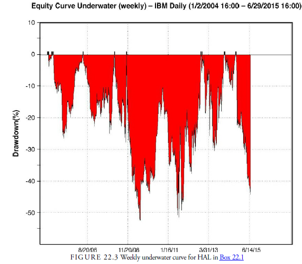
The second type of graph used to look at system performance is the underwater curve chart. An example of this type of chart is shown in Figure 22.3. This displays the drawdown from each successively higher peak in equity. It is calculated in percentages and gives a representation not only of how much drawdown occurred, but also of how much time passed until equity recovered from that drawdown. As Figure 22.3 shows, the maximum percentage drawdown in the initial HAL system was a little over 90% of the original capital of $30,000. This chart helps us see that a major problem with the system is not only the size of the drawdowns but also the time it takes for the system to recover. In Box 22.2, we outline a method for improving the system.
Box 22.2 Upgrade in the HAL
Now it is time to upgrade our system based on the results of our initial testing. We first optimize the parameters of the given variables to see if there is a possibility of an improved system just by changing the parameters. This is the first step, and it showed that with curvefitting, the net profit of over $35,000 was possible versus the loss incurred without adjustments. The second step is that we run a walk-forward test of the results and arrive at a system that we can expect to work in the near future. This is the one we report on here.
The changes made to HAL are threefold. First, we include a filter that will prevent the system from trading when the market is dull. We do this using a requirement that the ADX be higher than its predecessor some unknown number of days prior. We use the ADX because it is a measure of trend and we don’t want to play if there is no trend. There are other configurations of the ADX as a filter, but this is the one that worked best with HAL. Second, we add a percentage protective stop to lower the number of losses that accumulated time and loss while waiting for a buy signal. Third, we run optimizations on the parameters of ADX length, ADX lookback, CCI length, and upper and lower signal levels. The optimal results, using the perfect profit correlation as the objective function, were then run through a walk- forward optimizer to see which combination of parameters has the most likely chance of profiting in the next year.
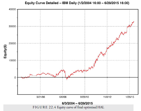
Look at how the system improves with the additions. Figure 22.4 shows the new equity curve for the system. Notice how smooth the curve is now. Net profit has increased from $2,000 to $31,000. The number of trades has decreased because of the ADX filter; the eliminated trades were obviously losers because the percentage of winners increased. The profit per trade is now high enough to withstand any extra trading costs, and the profit factor is now above the 2.00 standard threshold for a favorable system. The higher monthly return versus the standard deviation is well below the 5.00 normal ratio and explains why the equity curve is so smooth.
Do not use this system as it stands in any stock. It is presented only as an example of the process of looking for parameters, variables, and rules in a system development.
However, we hope that you can see the process of developing a reliable and profitable system and some of the types of adjustments that can be applied to systems—especially the use of stops—to improve performance and reduce risk. System development is a difficult and timeconsuming task.
Box 22.3 What is a Good Trading System?
In his book Beyond Technical Analysis, Tushar Chande discusses the characteristics of a good trading system. Chande’s Cardinal Rules for a good trading system are the following:
-
- Positive expectation—Greater than 13% annually.
- Small number of robust trading rules—Less than ten each is best for entry and exit rules.
- Able to trade multiple markets—Can use baskets for determining parameters, but rules should work across similar markets, different stocks, different commodities futures, and so on.
- Incorporates good risk control—Minimum risk as defined by drawdown should not be more than 20% and should not last more than nine months.
- Fully mechanical—No second-guessing during operation of the system.
Source: Kirkpatrick II Charles D., Dahlquist Julie R. (2015), Technical Analysis: The Complete Resource for Financial Market Technicians, FT Press; 3rd edition.
You have brought up a very superb details , regards for the post.