Lowess Smoothing by using Stata

Lowess smoothing, already demonstrated without explanation at several points in this book, is a very useful tool for nonparametric regression. Nonparametric regression methods generally do not yield an explicit regression equation, and do not require the analyst to specify a relationship’s functional form in advance. Instead, they help to explore the data with an open mind. This process can uncover unexpected and interesting results.

The lowess and graph twoway lowess commands both accomplish lowess smoothing (for locally weighted scatterplot smoothing). The lowess command with generate option can save predicted values. graph twoway lowess has advantages of simplicity, and follows the familiar syntax and overlay capabilities of the graph twoway family. For a basic example we graph global temperature anomalies using dataset global3.dta, introduced in Chapter 2.

Global temperature anomalies from 1880 through 2011 show considerable variation. From one month or year to the next, it would be impossible to tell whether the longer-term climate is warming, cooling or staying about the same. Lowess smoothing provides a view of longer-term change underneath rapid monthly fluctuations. Figure 8.1 draws a line plot of temperature against elapsed date (twoway line temp edate), then overlays this with a lowess smoothed curve with bandwidth .3, using a thicker line for emphasis (lowess temp edate, bw(.3) lwidth(thick)). Type help linewidthstyle for other choices of line width.

The lowess curve in Figure 8.1 clearly shows stages of early 20th century warming (especially 1920-1940), mid-century cooling, and modern rapid warming (post-1970) comprising the signature pattern of global climate change. The same stages appeared in local data on Lake Winnipesaukee ice-out dates, graphed in Figure 3.26 of Chapter 3.

Lowess predicted (smoothed) y values for n observations result from n weighted regressions. Let k represent the half-bandwidth, truncated to an integer. For each y_t , a smoothed value y- is obtained by weighted regression involving only those observations within the interval from i = max(1, i – k) through i = min(i + k, n). The jth observation within this interval receives weight Wj according to a tricube function:

A stands for the distance between x_t and its furthest neighbor within the interval. Weights equal 1 for Xj = Xj , but fall off to zero at the interval’s boundaries. See Chambers et al. (1983) or Cleveland (1993) for more discussion and examples of lowess methods.

lowess options include the following.

mean For running-mean smoothing. The default is running-line least squares smoothing.

noweight Unweighted smoothing. The default is Cleveland’s tricube weighting function.

bwidth( ) Specifies the bandwidth. Centered subsets of approximately bwidth x n observations are used for smoothing, except towards the endpoints where smaller, uncentered bands are used. The default is bwidth(.8).

logit Transforms smoothed values to logits.

adjust Adjusts the mean of smoothed values to equal the mean of the originaly variable;

like logit, adjust is useful with dichotomous y.

gen(newvar)         Creates newvar containing smoothed values of y.

nograph Suppresses displaying the graph.

addplot( ) Add other plots to the generated graph; see help addplot option .

lineopts( ) Affects the rendition of the smoothed line; see help cline options.

Because it requires n weighted regressions, lowess smoothing proceeds slowly with large samples.

Like other smoothing methods (or indeed, any model), lowess breaks the data into two parts: a smooth part such as the thick curve in Figure 8.1, and a rough part which is left over after subtracting the smooth from the data. Often the rough contains useful information as well. To illustrate we shift to a different atmospheric dataset on a multi-century timescale, containing measurements from the Greenland Ice Sheet 2 (GISP2) project described in Mayewski, Holdsworth and colleagues (1993) and Mayewski, Meeker and colleagues (1993). Researchers extracted and chemically analyzed an ice core representing more than 100,000 years of climate history. Greenlandsulfate.dta includes a very small fraction of this information: measured non­sea salt sulfate concentration and an index of Polar Circulation Intensity since the year 1500.

To retain more detail from this 271-point time series, we smooth with a relatively narrow bandwidth, only 5% of the sample. Figure 8.2 graphs the results for sulfate.

. graph twoway line sulfate year

|| lowess sulfate year, bwidth(.05) lwidth(medthick)

||   , ytitle(“SO{subscript:4} ion concentration, ppb”)

legend(label(1 “raw data”) label(2 “lowess smoothed”) position(11) ring(0) rows(2)))

Non-sea salt sulfate (SO₄) reached the Greenland ice after being injected into the atmosphere, chiefly by volcanoes or the burning of fossil fuels such as coal and oil. Both the smoothed and raw curves in Figure 8.2 convey information. The smoothed curve shows oscillations around a slightly rising mean from 1500 through the early 1800s. After 1900, fossil fuels drive the smoothed curve upward, with temporary setbacks after 1929 (the Great Depression) and the early 1970s (combined effects of the U.S. Clean Air Act, 1970; the Arab oil embargo, 1973; and subsequent oil price hikes). Most of the sharp peaks of the raw data have been identified with known volcanic eruptions such as Iceland’s Hekla (1970) or Alaska’s Katmai (1912).

After smoothing time series data, it is often useful to study the smooth and rough (residual) series separately. Below we use the lowess command to define two new variables: lowess- smoothed values of sulfate (smooth) and the residuals or rough values (rough) calculated by subtracting the smoothed values from the raw data.

. lowess sulfate year, bwidth(.05) gen(smooth)

. label variable smooth “SO4 ion concentration (smoothed)”

. gen rough = sulfate – smooth

. label variable rough “SO4 ion concentration (rough)”

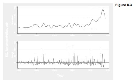
Figure 8.3 compares the smooth and rough time series in a pair of graphs annotated using text() options. Note the use of saving() options within each of the first two graph commands. These two graphs are then placed into one image with graph combine. In the combined graph, a common x-axis title is supplied: b1title(“Year”). b1 refers to the first bottom title. A combined graph does not know about x and y axis titles, but recognizes bottom (b1 and b2), left (11 and 12), top (t1 and t2) or right (r1 and r2) titles instead. In Figure 8.3 a common y-axis title is supplied as the first left-hand title, l1title(“SO{subscript:4} ion concentration, ppb”).

. graph twoway line smooth year, ylabel(0(50)150) xtitle(“”)

lwidth(medthick) lcolor(maroon) ytitle(“Smoothed”)

text(20 1540 “Renaissance”) text(20 1900 “Industrialization”)

text(90 1860 “Great Depression 1929”)

text(150 1935 “Oil Embargo 1973”)

saving(fig08_03a.gph, replace)

. graph twoway line rough year, ylabel(0(50)150) xtitle(“”)

ytitle(“Rough”) text(75 1630 “Awu 1640”, orientation(vertical))

text(120 1770 “Laki 1783”, orientation(vertical))

text(90 1805 “Tambora 1815”, orientation(vertical))

text(65 1902 “Katmai 1912”, orientation(vertical))

text(80 1960 “Hekla 1970”, orientation(vertical))

yline(0) saving(fig08_03b.gph, replace)

. graph combine fig08_03a.gph fig08_03b.gph, rows(2) b1title(“Year”)

l1title(“SO{subscript:4} ion concentration, ppb”)

Source: Hamilton Lawrence C. (2012), Statistics with STATA: Version 12, Cengage Learning; 8th edition.